Download
1 / 34
350 likes | 468 Views
Exponential Growth or Decay Function.

E N D
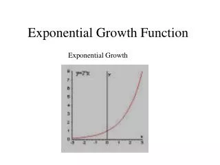
Exponential Growth or Decay Function In many situations that occur in ecology, biology, economics, and the social sciences, a quantity changes at a rate proportional to the amount present. In such cases the amount present at time t is a special function of t called an exponential growth or decay function.
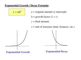
Exponential Growth or Decay Function Let y0 be the amount or number present at time t = 0. Then, under certain conditions, the amount present at any time t is modeled by where k is a constant.
DETERMINING AN EXPONENTIAL FUNCTION TO MODEL THE INCREASE OF CARBON DIOXIDE Example 1 Find an exponential function that gives the amount of carbon dioxide y inyear t. a. Solution Recall that the graph of the data points showed exponential growth, so the equation will take the form y = y0ekt. We must find the values of y0 and k. The data began with the year 1990, so to simplify our work we let 1990 correspond to t = 0, 1991 correspond to t = 1, and so on. Since y0 is the initial amount, y0 = 353 in 1990, that is, when t = 0.
DETERMINING AN EXPONENTIAL FUNCTION TO MODEL THE INCREASE OF CARBON DIOXIDE Example 1 Find an exponential function that gives the amount of carbon dioxide y inyear t. a. Solution Thus the equation is From the last pair of values in the table, we know that in 2275 the carbon dioxide level is expected to be 2000 ppm. The year 2275 corresponds to 2275 – 1990 = 285. Substitute 2000 for y and 285 for t and solve for k.
DETERMINING AN EXPONENTIAL FUNCTION TO MODEL THE INCREASE OF CARBON DIOXIDE Example 1 Solution Divide by 353. Take logarithms on both sides. In ex = x
DETERMINING AN EXPONENTIAL FUNCTION TO MODEL THE INCREASE OF CARBON DIOXIDE Example 1 Solution Multiply by ; rewrite. Use a calculator. A function that models the data is
DETERMINING AN EXPONENTIAL FUNCTION TO MODEL THE INCREASE OF CARBON DIOXIDE Example 1 b. Estimate the year when future levels of carbon dioxide will double the 1951 level of 280 ppm. Solution Let y = 2(280) = 560 in y = 353e.00609t , and find t. Divide by 353. Take logarithms on both sides.
DETERMINING AN EXPONENTIAL FUNCTION TO MODEL THE INCREASE OF CARBON DIOXIDE Example 1 In ex = x Multiply by ; Rewrite. Use a calculator. Since t = 0 corresponds to 1990, the 1951 carbon dioxide level will double in the 75th year after 1990, or during 2065.
FINDING DOUBLING TIME FOR MONEY Example 2 How long will it take for the money in an account that is compounded continuously at 3% interest to double? Solution Continuous compounding formula Let A = 2P and r = .03 Divide by P Take logarithms on both sides.
FINDING DOUBLING TIME FOR MONEY Example 2 How long will it take for the money in an account that is compounded continuously at 3% interest to double? Solution In ex = x Divide by .03 Use a calculator. It will take about 23 yr for the amount to double.
DETERMINING AN EXPONENTIAL FUNCTION TO MODEL POPULATION GROWTH Example 3 According to the U.S. Census Bureau, the world population reached 6 billion people on July 18, 1999, and was growing exponentially. By the end of 2000, the population had grown to 6.079 billion. The projected world population (in billions of people) t years after 2000, is given by the function defined by
DETERMINING AN EXPONENTIAL FUNCTION TO MODEL POPULATION GROWTH Example 3 a. Based on this model, what will the world population be in 2010? Solution Since t = 0 represents the year 2000, in 2010, t would be 2010 – 2000 = 10 yr. We must find (t) when t is 10. Let t = 10. According to the model, the population will be 6.895 billion at the end of 2010.
DETERMINING AN EXPONENTIAL FUNCTION TO MODEL POPULATION GROWTH Example 3 b. In what year will the world population reach 7 billion? Solution Let t = 7. Divide by 6.079 Take logarithms on both sides
DETERMINING AN EXPONENTIAL FUNCTION TO MODEL POPULATION GROWTH Example 3 b. In what year will the world population reach 7 billion? Solution In ex = x Divide by .0126; rewrite. Use a calculator. World population will reach 7 billion 11.2 yr after 2000, during the year 2011.
DETERMINING AN EXPONENTIAL FUNCTION TO MODEL RADIOACTIVE DECAY Example 4 If 600 g of a radioactive substance are present initially and 3 yr later only 300 g remain, how much of the substance will be present after 6 yr? Solution To express the situation as an exponential equation we use the given values to first find y0 and then find k.
DETERMINING AN EXPONENTIAL FUNCTION TO MODEL RADIOACTIVE DECAY Example 4 If 600 g of a radioactive substance are present initially and 3 yr later only 300 g remain, how much of the substance will be present after 6 yr? Solution Let y = 600 and t = 0. e0 = 1 Thus, y0 = 600 and the exponential equation y = y0ekt becomes
DETERMINING AN EXPONENTIAL FUNCTION TO MODEL RADIOACTIVE DECAY Example 4 Solution Now solve this exponential equation for k. Let y = 300 and t = 3. Divide by 600. Take logarithms on both sides.
DETERMINING AN EXPONENTIAL FUNCTION TO MODEL RADIOACTIVE DECAY Example 4 Solution In ex = x Divide by 3. Use a calculator.
DETERMINING AN EXPONENTIAL FUNCTION TO MODEL RADIOACTIVE DECAY Example 4 Solution Thus, the exponential decay equation is y = 600e–.231t . To find the amount present after 6 yr, let t = 6. After 6 yr, about 150 g of the substance will remain.
Half Life Analogous to the idea of doubling time is half-life, the amount of time that it takes for a quantity that decays exponentially to become half its initial amount.
SOLVING A CARBON DATING PROBLEM Example 5 Carbon 14, also known as radiocarbon, is a radioactive form of carbon that is found in all living plants and animals. After a plant or animal dies, the radiocarbon disintegrates. Scientists can determine the age of the remains by comparing the amount of radiocarbon with the amount present in living plants and animals. This technique is called carbon dating. The amount of radiocarbonpresent after t years is given by where y0 is the amount present in living plants and animals.
SOLVING A CARBON DATING PROBLEM Example 5 a. Find the half-life. Solution If y0 is the amount of radiocarbon present in a living thing, then ½ y0 is half this initial amount. Thus, we substitute and solve the given equation for t. Let y = ½ y0 .
SOLVING A CARBON DATING PROBLEM Example 5 a. Find the half-life. Solution Let y = ½ y0 . Divide by y0. Take logarithms on both sides.
SOLVING A CARBON DATING PROBLEM Example 5 a. Find the half-life. Solution In ex = x Divide by –.0001216 Use a calculator. The half-life is about 5700 yr.
SOLVING A CARBON DATING PROBLEM Example 5 b. Charcoal from an ancient fire pit on Java contained ¼ the carbon 14 of a living sample of the same size. Estimate the age of the charcoal. Solution Solve again for t, this time letting the amount y = ¼ y0. Given equation. Let y = ¼ y0 .
SOLVING A CARBON DATING PROBLEM Example 5 Solution Divide by y0 . Take logarithms on both sides In ex = x; divide by −.0001216 Use a calculator. The charcoal is about 11,400 yr old.
MODELING NEWTON’S LAW OF COOLING Example 6 Newton’s law of cooling says that the rate at which a body cools is proportional to the difference C in temperature between the body and the environment around it. The temperature (t) of the body at time t in appropriate units after being introducedinto an environment having constant temperature T0 is where C and k are constants.
MODELING NEWTON’S LAW OF COOLING Example 6 A pot of coffee with a temperature of 100°C is set down in a room with a temperature of 20°C. The coffee cools to 60°C after 1 hr. a. Write an equation to model the data. Solution We must find values for C and k in the formula for cooling. From the given information, when t = 0, T0 = 20, and the temperature of the coffee is (0) = 100. Also, when t = 1, (1) = 60. Substitute the first pair of values into the equation along with T0 =20.
MODELING NEWTON’S LAW OF COOLING Example 6 a. Write an equation to model the data. Solution Given formula Let t = 0, (0) = 100, and T0 = 20. e0 = 1 Subtract 20. Thus,
MODELING NEWTON’S LAW OF COOLING Example 6 Solution Now use the remaining pair of values in this equation to find k. Given formula Let t = 1, (1) = 60. Subtract 20. Divide by 80. Take logarithms on both sides.
MODELING NEWTON’S LAW OF COOLING Example 6 Solution Now use the remaining pair of values in this equation to find k. In ex = x Thus,
MODELING NEWTON’S LAW OF COOLING Example 6 b. Find the temperature after half an hour. Solution To find the temperature after ½ hr, let t = ½ in the model from part (a). Model from part (a) Let t = ½ .
MODELING NEWTON’S LAW OF COOLING Example 6 c. How long will it take for the coffee to cool to 50°C? Solution To find how long it will take for the coffee to cool to 50°C, let (t) = 50. Let (t) = 50. Subtract 20. Divide by 80.
MODELING NEWTON’S LAW OF COOLING Example 6 c. How long will it take for the coffee to cool to 50°C? Solution To find how long it will take for the coffee to cool to 50°C, let (t) = 50. Take logarithms on both sides. In ex = x