Download
1 / 56
560 likes | 561 Views
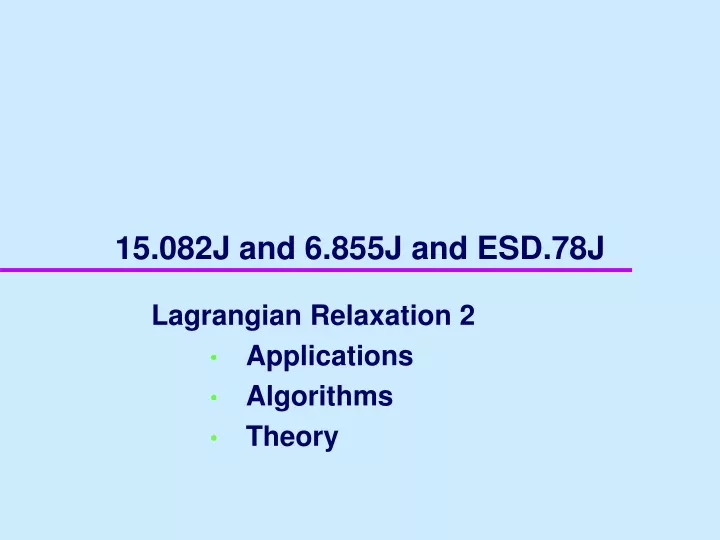
15.082J and 6.855J and ESD.78J. Lagrangian Relaxation 2 Applications Algorithms Theory. Lagrangian Relaxation and Inequality Constraints. z * = Min cx subject to A x ≤ b, (P * ) x ∈ X. L( μ ) = Min cx + μ ( A x - b) (P * ( μ ))

E N D
15.082J and 6.855J and ESD.78J Lagrangian Relaxation 2 Applications Algorithms Theory
Lagrangian Relaxation and Inequality Constraints z* = Min cx subject to Ax ≤ b, (P*) x ∈ X. L(μ) = Min cx + μ(Ax - b) (P*(μ)) subject to x ∈ X, Lemma. L(μ) ≤ z* for μ≥ 0. The Lagrange Multiplier Problem: maximize (L(μ) : μ≥ 0). Suppose L* denotes the optimal objective value, and suppose x is feasible for P* and μ≥ 0. Then L(μ) ≤ L* ≤ z* ≤ cx.
Lagrangian Relaxation and Equality Constraints z* = Min cx subject to Ax = b, (P*) x ∈ X. L(μ) = Min cx + μ(Ax - b) (P*(μ)) subject to x ∈ X, Lemma. L(μ) ≤ z* for all μ ∈ Rn The Lagrange Multiplier Problem: maximize (L(μ) : μ ∈ Rn). Suppose L* denotes the optimal objective value, and suppose x is feasible for P* and μ≥ 0. Then L(μ) ≤ L* ≤ z* ≤ cx.
Generalized assignment problem ex. 16.8 Ross and Soland [1975] 1 1 2 2 3 3 4 4 5 aij = the amount of processing time of job i on machine j xij = 1 if job i is processed on machine j = 0 otherwise Job i gets processed. Machine j has at most dj units of processing Set I of jobs Set J of machines
Generalized assignment problem ex. 16.8 Ross and Soland [1975] Minimize (16.10a) (16.10b) (16.10c) (16.10d) Generalized flow with integer constraints. Class exercise: write two different Lagrangian relaxations.
customer potential facility Facility Location Problem ex. 16.9Erlenkotter 1978 • Consider a set J of potential facilities • Opening facility j ∈ J incurs a cost Fj. • The capacity of facility j is Kj. • Consider a set I of customers that must be served • The total demand of customer i is di. • Serving one unit of customer i’s from location j costs cij.
Class Exercise Formulate the facility location problem as an integer program. Assume that a customer can be served by more than one facility. Suggest a way that Lagrangian Relaxation can be used to help solve this problem. Let xij be the amount of demand of customer i served by facility j. Let yj be 1 if facility j is opened, and 0 otherwise.
Solving the Lagrangian Multiplier Problem Approach 1: represent the LP feasible region as the convex combination of corner points. Then use a constraint generation approach. Approach 2: subgradient optimization
(1,1) 2 4 (1,7) (1,10) (2,3) (10,1) 1 6 (1,2) (5,7) (10,3) (2,2) 5 3 (12,3) The Constrained Shortest Path Problem Find the shortest path from node 1 to node 6 with a transit time at most 14.
Constrained Shortest Paths: Path Formulation Given: a network G = (N,A) cij cost for arc (i,j) c(P) cost of path P tij traversal time for arc (i,j) T upper bound on transit times. t(P) traversal time for path P Pset of paths from node 1 to node n Min c(P) s.t. t(P) ≤ T P ∈ P L(μ) = Min c(P) + μ t(P) - μT s.t. P ∈ P Lagrangian Constrained Problem
The Lagrangian Multiplier Problem Step 0. Formulate the Lagrangian Problem. L(μ) = Min c(P) + μ t(P) - μT s.t. P ∈ P L(μ) = Max w s.t w ≤ c(P) + μ t(P) – μT for all P ∈ P Step 1. Rewrite as a maximization problem L* = max {L(μ): μ ≥ 0} = = Max w s.t w ≤ c(P) + μ t(P) – μT for all P ∈ P μ ≥ 0 Step 2. Write the Lagrangian multiplier problem
Max { w: w ≤ c(P) + μ t(P) – μT ∀P ∈ P, and μ ≥ 0} 1-3-4-6 1-2-4-6 1-3-4-5-6 1-2-4-5-6 1-2-5-6 1-3-2-4-6 1-3-2-4-5-6 1-3-2-5-6 L* = max (L(μ): μ ≥ 0) 1-3-5-6 Paths 30 20 10 Composite Cost 0 -10 0 1 2 3 4 5 Lagrange Multiplier μ Figure 16.3 The Lagrangian function for T = 14. 15
The Restricted Lagrangian P : the set of paths from node 1 to node n S ⊆ P : a subset of paths L* = max w s.t w ≤ c(P) + μ t(P) –T for all P ∈ P μ ≥ 0 L*S = max w s.t w ≤ c(P) + μ t(P) – μT for all P ∈ S μ ≥ 0 Restricted Lagrangian Multiplier Problem Lagrangian Multiplier Problem If L(μ) = L*S then L(μ) = L*. L(μ) ≤ L* ≤ L*S Optimality Conditions
Constraint Generation for Finding L* Let Path(μ) be the path that optimizes the Lagrangian. Let Multiplier(S) be the value of μ that optimizes LS(μ). M is some large number Initialize: S := {Path(0), Path(M)} μ := Multiplier(S), Yes Is L(μ) = L*S? Quit. L(μ) = L* No S := S ∪ Path(μ)
3 + 18 μ 1-2-4-6 (2.1, 40.8) 24 + 8 μ 1-3-5-6 We start with the paths 1-2-4-6, and 1-3-5-6 which are optimal for L(0) and L(∞). Paths 30 20 10 Composite Cost 0 -10 0 1 2 3 4 5 Lagrange Multiplier μ 18
Set μ = 2.1 and solve the constrained shortest path problem The optimum path is 1-3-2-5-6 3.2 15 + 10 μ 2 4 15.7 22 8.3 12.1 1 6 5.2 19.7 16.3 6.2 5 3 18.3
1.5, 9 15 - 4 μ 1-3-2-5-6 Path(2.1) = 1-3-2-5-6. Add it to S and reoptimize. Paths 30 3 + 4 μ 1-2-4-6 20 10 Composite Cost 0 24 - 6 μ 1-3-5-6 -10 0 1 2 3 4 5 Lagrange Multiplier μ 20
Set μ = 1.5 and solve the constrained shortest path problem The optimum path is 1-2-5-6. 2.5 2 4 11.5 16 6.5 11.5 1 6 4 15.5 14.5 5 5 3 16.5
5 + μ 1-2-5-6 2, 7 Add Path 1-2-5-6 and reoptimize Paths 30 3 + 4 μ 1-2-4-6 20 10 Composite Cost 0 15 - 4 μ 1-3-2-5-6 24 - 6 μ 1-3-5-6 -10 0 1 2 3 4 5 Lagrange Multiplier μ 22
Set μ = 2 and solve the constrained shortest path problem The optimum paths are 1-2-5-6 and1-3-2-5-6 3 2 4 15 21 8 12 1 6 5 19 16 6 5 3 18
2, 7 There are no new paths to add. μ*is optimal for the multiplier problem Paths 30 3 + 4 μ 1-2-4-6 20 5 + μ 1-2-5-6 10 Composite Cost 0 15 - 4 μ 1-3-2-5-6 24 - 6 μ 1-3-5-6 -10 0 1 2 3 4 5 Lagrange Multiplier μ 24
Mental Break Where did the name Gatorade come from? The drink was developed in 1965 for the Florida Gators football team. The team credits in 1967 Orange Bowl victory to Gatorade. What percentage of people in the world have never made or received a phone call? 50% What causes the odor of natural gas? Natural gas has no odor. They add the smell artificially to make leaks easy to detect.
Mental Break What is the most abundant metal in the earth’s crust? Aluminum How fast are the fastest shooting stars? Around 150,000 miles per hour. The Malaysian government banned car commercials starring Brad Pit. What was their reason for doing so? Brad Pitt was not sufficiently Asian looking. Using a Caucasian such as Brad was considered “an insult to Asians.”
Towards a general theory Next: a way of generalizing Lagrangian Relaxation for the time constrained shortest path problem to LPs in general. Key fact: bounded LPs are optimized at extreme points.
Extreme Points and Optimization Paths ⇔ Extreme Points Optimizing over paths ⇔ Optimizing over extreme points If an LP region is bounded, then there is a minimum cost solution that occurs at an extreme (corner) point)
Convex Hulls and Optimization: The convex hull of a set X of points is the smallest LP feasible region that contains all points of X. The convex hull will be denoted as H(X) . Min cx s.t x ∈ X Min cx s.t. x ∈ H(X) `
Convex Hulls and Optimization: Let S = {x : Ax = b, x ≥ 0}. Suppose that S has a bounded feasible region. Let Extreme(S) be the set of extreme points of S. Min cx s.t Ax = b x ≥ 0 Min cx s.t. x ∈ Extreme(S) `
Convex Hulls Suppose that X = {x1, x2, …, xK} is a finite set. Vector y is a convex combination of X = {x1, x2, …, xK} if there is a feasible solution to The convex hull of X is H(X) = { x : x can be expressed as a convex combination of points in X.}
Lagrangian Relaxation and Inequality Constraints z* = min cx subject to Ax ≤ b, (P) x ∈ X. L(μ) = min cx + μ(Ax - b) (P(μ)) subject to x ∈ X. L* = max (L(μ) : μ≥ 0). So we want to maximize over μ, while we are minimizing over x.
An alternative representation Suppose that X = {x1, x2, x3, …, xK}. Possibly K is exponentially large; e.g., X is the set of paths from node s to node t. L(μ) = min cx + μ(Ax - b) = (c + μA)x - μb subject to x ∈ X. L(μ) = min {(c + μA)xk - μb : k = 1 to K} L(μ) = max w s.t. w ≤ (c + μA)xk - μb for all k
The Lagrange Multiplier Problem L* = max w s.t. w ≤ (c + A)xk - μb for all k ∈ [1,K] μ ∈ Rn Suppose that S ⊆ [1,K] For a fixed value μ L*S(μ) = max w s.t. w ≤ (c + μA)xk - μb for all k ∈ S L*S = max w s.t. w ≤ (c + μA)xk - μb for all k ∈ S μ ∈ Rn
Constraint Generation for Finding L* Suppose that Extreme(μ) optimizes the Lagrangian. Let Multiplier(S) be the value of μ that optimizes LS(μ). Initialize with a set S of extreme points of X. μ := Multiplier(S), Yes Is L(μ) = L*S? Quit. L(μ) = L* No S := S ∪ Extreme(μ)
1-3-4-6 1-2-4-6 1-3-4-5-6 1-2-4-5-6 1-2-5-6 1-3-2-4-6 1-3-2-4-5-6 1-3-2-5-6 L* = max (L(μ): μ ≥ 0) 1-3-5-6 Paths 30 20 10 Composite Cost 0 -10 0 1 2 3 4 5 Lagrange Multiplier μ Figure 16.3 The Lagrangian function for T = 14. 36
3 + 18 μ 1-2-4-6 2.1, 40.8 24 + 8 μ 1-3-5-6 We start with the paths 1-2-4-6, and 1-3-5-6 which are optimal for L(0) and L(μ). Paths 30 20 10 Composite Cost 0 -10 0 1 2 3 4 5 Lagrange Multiplier μ 37
1.5, 9 15 - 4 μ 1-3-2-5-6 Add Path 1-3-2-5-6 and reoptimize Paths 30 3 + 4 μ 1-2-4-6 20 10 Composite Cost 0 24 - 6 μ 1-3-5-6 -10 0 1 2 3 4 5 Lagrange Multiplier μ 38
5 + μ 1-2-5-6 2, 7 Add Path 1-2-5-6 and reoptimize Paths 30 3 + 4 μ 1-2-4-6 20 10 Composite Cost 0 15 - 4 μ 1-3-2-5-6 24 - 6 μ 1-3-5-6 -10 0 1 2 3 4 5 Lagrange Multiplier μ 39
2, 7 There are no new paths to add. μ*is optimal for the multiplier problem Paths 30 3 + 4 μ 1-2-4-6 20 5 + μ 1-2-5-6 10 Composite Cost 0 15 - 4 μ 1-3-2-5-6 24 - 6 μ 1-3-5-6 -10 0 1 2 3 4 5 Lagrange Multiplier μ 40
Subgradient optimization Another major solution technique for solving the Lagrange Multiplier Problem is subgradient optimization. Based on ideas from non-linear programming. It converges (often slowly) to the optimum. See the textbook for more information.
Application Embedded Network Structure Networks with side constraints minimum cost flowsshortest paths Traveling Salesman Problem assignment problemminimum cost spanning tree Vehicle routing assignment problemvariant of min cost spanning tree Network design shortest paths Two-duty operator scheduling shortest pathsminimum cost flows Multi-timeproduction planning shortest paths / DPsminimum cost flows
Interpreting L* • For LP’s, L* is the optimum value for the LP • Relation of L* to optimizing over a convex hull
Lagrangian Relaxation applied to LPs z* = min cx s.t. Ax = b Dx = d x ≥ 0 LP L(μ) = min cx + μ(Ax – b) s.t. Dx = d x ≥ 0 LP(μ) L* = max L(μ) s.t. μ ∈ Rn LMP Theorem 16.6 If -∞ < z* < ∞, then L* = z*.
On the Lagrange Multiplier Problem Theorem 16.6 If -∞ < z* < ∞, then L* = z*. Does this mean that solving the Lagrange Multiplier Problem solves the original LP? No! It just means that the two optimum objective values are the same. Sometimes it is MUCH easier to solve the Lagrangian problem, and getting an approximation to L* is also fast.
Property 16.7 • The set H(X) is a polyhedron, that is, it can be expressed as H(X) = {x : Ax ≤ b} for some matrix A and vector b. • Each extreme point of H(X) is in X. If we minimize {cx : x ∈ H(X)}, the optimum solution lies in X. • Suppose X ⊆ Y = {x : Dx ≤ c and x ≥ 0}. Then H(X) ⊆ Y.
Relationships concerning LPs z* = Min cx s.t Ax = b x ∈ X v* = Min cx s.t Ax = b x ∈ H(X) Original Problem X replaced by H(X) L(μ) = Min cx + μ(Ax – b) s.t x ∈ X v(μ) = Min cx + μ(Ax – b) s.t x ∈ H(X) Lagrangian X replaced by H(X) L(μ) = v(μ) ≤ v* ≤ z*
max x1s.t. x1≤ 6 x ∈ X is different from max x1s.t. x1≤ 6 x ∈ H(X) x1
Relationships concerning LPs z* = Min cx s.t Ax = b x ∈ X v* = Min cx s.t Ax = b x ∈ H(X) L(μ) = Min cx + μ(Ax – b) s.t x ∈ X v(μ) = Min cx + μ(Ax – b) s.t x ∈ H(X) L* = max {L(μ) : μ ∈ Rn } v* = max {v(μ) : μ ∈ Rn } L(μ) = v(μ) ≤ L* = v* ≤ z* Theorem 16.8. L* = v*.
Illustration min - x1s.t. x1≤ 6 x ∈ H(X) Lagrangianmin - x1 + μ(x1 – 6) = (μ-1)x1 - 6μ s.t. x ∈ X x1 1 6 11 L(μ) = (μ-1) - 6μ = -5μ -1 if μ ≥ 1 L* = -6 L(μ) = 11(μ-1) - 6μ = 5μ -11 if μ ≤ 1