Download
1 / 24
240 likes | 244 Views
This lecture covers topics such as catalog cross-matching, resolving sources, selection biases, luminosity functions, and the difference between volume-limited and flux-limited surveys. Python tutorials and modules are also discussed.

E N D
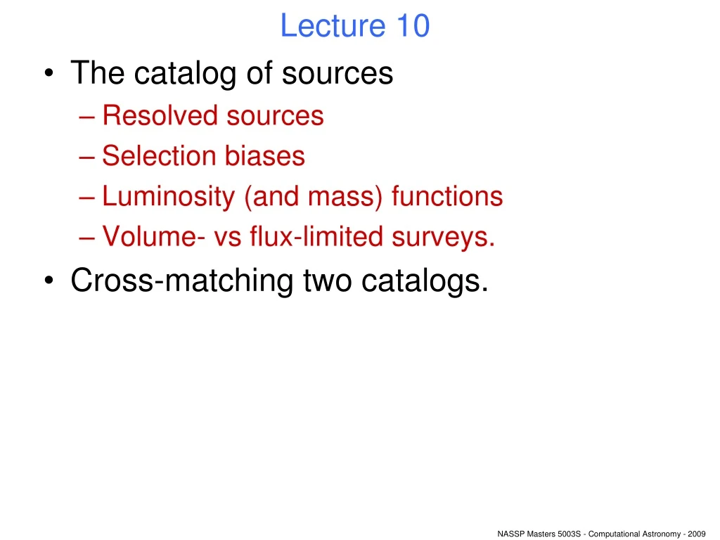
Lecture 10 • The catalog of sources • Resolved sources • Selection biases • Luminosity (and mass) functions • Volume- vs flux-limited surveys. • Cross-matching two catalogs.
Python and tut oddments • The module cPickle offers a useful way to save to disk file python-generated data of arbitrary format. • See http://www.python.org/doc/2.5/lib/module-cPickle.html • This can save you having to run a whole MC again just to check the details of a plot! • I see that pyfits is set up to deliver numpy arrays on the NASSP machines. (It only returns Numarray objects on Astronomy computers it seems.) • Assessment: let us take ‘code must run’ to mean ‘it must run on NASSP machines.’ • If I claim you code won’t run, and you think I am wrong, by all means protest!
Detecting resolved sources. • Our earlier assumption that we knew the form of S is no longer true. • Some solutions: • Combine results of several filterings. (Crudely done in XMM.) • But, ‘space’ of possible shapes is large. • Difficult to calculate nett sensitivity. • Wavelet methods.
Wavelet example F Damiani et al (1997) Raw data Wavelet smoothed Multi-scale wavelets can be chosen to return best-fit ellipsoids.
Selection biases • Fundamental aim of most surveys is to obtain measurements of an ‘unbiased sample’ of a type of object. • Selection bias happens when the survey is more sensitive to some classes of source than others. • Eg, intrinsically brighter sources, obviously. • Problem is even greater for resolved sources. • Note: ‘resolved’ does not just mean in spatial terms. Eg XMM or (single-dish HI surveys) in which most sources are unresolved spatially, but well resolved spectrally.
Examples • Optical surveys of galaxies. Easiest detected are: • The brightest (highest apparent magnitude). • Edge-on spirals. • HI (ie, 21 cm radio) surveys of galaxies. Easiest detected are: • Those with most HI mass (excludes ellipticals). • Those which don’t ‘fill the beam’ (ie are unresolved). • Note: where sources are resolved, detection sensitivity tends to depend more on surface brightness than total flux.
Full spatial information • Q: We have a low-flux source - how do we tell whether it is a high-luminosity but distant object, or a low-luminosity nearby one? • A: Various distance measures. • Parallax - only for nearby stars – but Gaia will change that. • Special knowledge which lets us estimate luminosity (eg Herzsprung-Russell diagram). • Redshift => distance via the Hubble relation. This is probably the most widely used method for extragalactic objects.
Luminosity function P Kroupa (1995) • Frequency distribution of luminosity (luminosity = intrinsic brightness). • The faint end is the hardest to determine. • Stars – how many brown dwarfs? • Galaxies – how many dwarfs? • Distribution for most objects has a long faint-end ‘tail’. • Schechter functions. P Schechter (1976)
HI mass function • Red shift is directly measured. • Flux is proportional to mass of neutral hydrogen (HI). • Hence: usual to talk about HI mass function rather than luminosity function. S E Schneider (1996) FYI, HI is pronounced ‘aitch one’.
Relation to logN-logS • Just as flux S is related to luminosity L and distance D by • So is the logN-logS – or, to be more exact, the number density as a function of flux, n(S) - a convolution between the luminosity function n(L) and the true spatial distribution n(D). • BUT… • The luminosity function can change with age – that is, with distance! (And with environment.) SαL/D2
Volume- vs flux-limited surveys • Information about the distance of sources allows one to set a distance cutoff, within which one estimates the survey is reasonably complete (ie, nearly all the available sources are detected). • Such a survey is called volume-limited. It allows the luminosity (or mass) function to be estimated without significant bias. • However, there may be few bright sources. • Allow everything in, and you have a flux-limited survey. • Many more sources => better stats; but biased (Malmquist bias).
Malmquist bias Line of constant flux
Malmquist bias Line of constant flux
Catalog cross-matching • It sometimes happens that you have 2 lists of objects, which you want to cross-match. • Maybe the lists are sources observed at different frequencies. • The situation also arises in simulations. • I’ll deal with the simulations situation first, because it is easier. • So: we start with a bunch of simulated sources. Let’s keep it simple and assume they all have the same brightness. • We add noise, then see how many we can find.
Catalog cross-matching • In order to know how well our source-detection machinery is working, we need to match each detection with one of the input sources. • How do we do this? • How do we know the ‘matched’ source is the ‘right one’? CAVEAT: ...I haven’t done a rigorous search of the literature yet – these are just my own ideas.
Catalog cross-matching Black: simulated sources Red: 1 of many detections (with 68% confidence interval). This case seems clear.
Catalog cross-matching But what about these cases? No matches inside confidence interval. Too many matches inside confidence interval.
Catalog cross-matching Or these? Is any a good match? Which is ‘nearest’?
Catalog cross-matching • My conclusion: • The shape of the confidence intervals affects which source is ‘nearest’. • The size of the confidence intervals has nothing to do with the probability that the ‘nearest’ match is non-random. • ‘Nearest neighbour’ turns out to be a slipperier concept than we at first think. To see this, imagine that we have now 1 spatial dimension and 1 flux dimension:
Catalog cross-matching Which is the best match??? Source 5? Or source 8? This makes more sense. Let’s then define r as: 9 8 7 6 5 4 S S 9 8 2 3 6 7 5 1 4 2 3 1 1 1 x x
Catalog cross-matching • As for the probability... well, what is the null hypothesis in this case? • Answer: that the two catalogs have no relation to each other. • So, we want the probability that, with a random distribution of the simulated sources, a source would lie as close or closer to the detected source than rnearest. • This is given by: • where ρ is the expected density of sim sources and V is the volume inside rnearest. Pnull = 1 – exp(-ρV)
Catalog cross-matching • So the procedure for matching to a simulated catalog is: • For each detection, find the input source for which r is smallest. • Calculate the probability of the null hypothesis from Pnull = 1 – exp(-ρV). • Discard those sources for which Pnull is greater than a pre-decided (low) cutoff. • What about the general situation of matching between different catalogs?
Catalog cross-matching ASCA data – M Akiyama et al (2003) Maybe a Bayesian approach would be best? Interesting area of research.