Download
1 / 20
200 likes | 206 Views
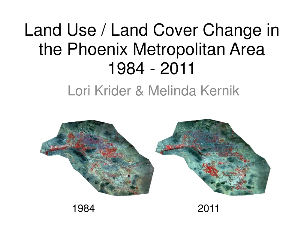
Land Use / Land Cover Change in the Phoenix Metropolitan Area 1984 - 2011. Lori Krider & Melinda Kernik. 1984. 2011. Why Phoenix? One of 10 fastest growing cities from 1990 - 2000 (Perry & Mackun, 2001) Arid regions with high population are water stressed

E N D
Land Use / Land Cover Change in the Phoenix Metropolitan Area1984 - 2011 Lori Krider & Melinda Kernik 1984 2011
Why Phoenix? • One of 10 fastest growing cities from 1990 - 2000 (Perry & Mackun, 2001) • Arid regions with high population are water stressed • Water use is reflected by how the land is used and managed • How is the landscape changing and how does this effect water use? Introduction
Use remote sensing software to assess land use / land cover change in Phoenix from 1984 – 2011 • Expect to see dramatic changes due to rapid population growth • Increase in urban and suburban areas (sprawl) • Increase in cultivated areas on edges of metropolitan area • Decrease in natural vegetation Objective
Objective • Study Area • Phoenix-Mesa Metropolitan Area • South-central Arizona • 16,200 km2 • Phoenix, Mesa, Tempe, Chandler, Gilbert, Scottsdale, Glendale, Sun City, Peoria, and Avondale Google Maps
Tools: ERDAS IMAGINE 2011, USGS GLOVIS, ArcGIS 10, Google MapsTM and Google EarthTM • Materials: Landsat TM images from 1984 and 2011 (two from each year, 30 m res., 7 bands, June), 2006 NLCD • Pre-classification processing • Stack bands, mosaic and crop images for each year • View NLCD • Unsupervised classification (5, 6 & 7 classes) Preparation
Supervised classification • Anderson Hierarchical Classification (levels 1 and 2) • Altered, unaltered, developed and water • Altered • Human-assisted: healthy and stressed crops, golf courses • Uncultivated: fields not reflecting in IR • Unaltered • Natural: upland and scrub/shrub (not in IR) • Hydrophillic vegetation: depressional vegetation often associated with water (in IR) • Water: lakes, rivers and large golf course water hazards • Developed • suburban (dwellings) & urban/roads (commercial/industrial) Analysis
Analysis • Training Areas • 15 - 45 • Why? • Errors in first run with less training areas • Combination of smaller category classes (i.e. healthy crop + stressed crop) • Reduce confusion and capture variety • Change Detection • Thematic: 1984 -> 2011 • Difference • to identify areas of significant change and overall patterns • 10, 20, and 30% thresholds
Post-classification • Accuracy Assessment • stratified random • same mosaics as reference • added Google MapsTM for 2011 • switched "trainers" • 140 reference points (20 per class) http://www.cartoonstock.com/directory/b/bad_appraisal.asp
1984 2011
Thematic Change Detection Purple: Change to Suburban Light Blue: Change to Urban
Purple = changed to Suburban Blue = changed to Urban
Green = more than 20% increase in NIR Blue = more than 20% decrease in NIR
Limitations! 2011 1984
For future classifications: • Clip to the smallest possible boundaries • More ontological classes = more classification confusion • Complications using 30m resolution images for reference data and the same image. • Use this technique, to generate water infrastructure policy for Phoenix …probably not
References • Perry, M. J. & P. J. Mackun. Population Change and Distribution 1990 - 2000: Census 2000 Brief. April 2011. United States Census Bureau. 12 Nov. 2011. <http://www.census.gov/prod/2011pubs/c2kbr01-2.pdf>.