Download
1 / 40
400 likes | 513 Views
Croucher ASI on Frontiers in Computational Methods and Their Applications in Physical Sciences Dec. 6 - 13, 2005 The Chinese University of Hong Kong.

E N D
Croucher ASI on Frontiers in Computational Methods and Their Applications in Physical Sciences Dec. 6 - 13, 2005 The Chinese University of Hong Kong The Search for Spin-waves in Iron Above Tc:Spin Dynamics SimulationsX. Tao, D.P.L., T. C. Schulthess*, G. M. Stocks* * Oak Ridge National Lab • Introduction What’s interesting, and what do we want to do? • Spin Dynamics Method • Results • Static properties • Dynamic structure factor • Conclusions
Iron (Fe) has had a great effect on mankind: N S Our current interest is in the magnetic properties
The controversy about paramagnetic Fe: Do spin waves persist aboveTc?
The controversy about paramagnetic Fe: Do spin waves persist aboveTc? Experimentally (triple-axis neutron spectrometer) ORNL: Yes, spin waves persist to 1.4Tc BNL: No
The controversy about paramagnetic Fe: Do spin waves persist aboveTc? Experimentally (triple-axis neutron spectrometer) ORNL: Yes, spin waves persist to 1.4Tc BNL: No Theoretically What is the spin-spin correlation length for Fe above Tc? Are there propagating magnetic excitations?
What is a spin wave? Consider ferromagnetic spins on a 1-d lattice (a) The ground state(T=0 K) (b) A spin-wave state Spin-waves are propagating excitations with characteristic wavelength and velocity
Facts about BCC iron Electronic configuration 3d64s2 Tc = 1043 K (experiment, pure Fe) TBCC FCC = 1183 K (BCC FCC eliminated with addition of silicon)
Heisenberg Hamiltonian Shells of neighbors N = 2 L3 spins on an LLL BCC lattice |Sr| = 1 ,classical spins Spin magnetic moments absorbed into J J = Jr,r’where is the neighbor shell
Exchange parameters J First principles electronic structure calculations (T. Schulthess, private communication)
Exchange parameters J (cont’d.) T = 0.3 Tc (room temperature) BCC Fe dispersion relation Nearest neighbors only Least squares fit After Shirane et al, PRL (1965)
(Spin dynamics) Simulation NATURE Theory Experiment (Neutron scattering)
Center for Stimulational PhysicsCenter for Simulated Physics
Center for Stimulational PhysicsCenter for Simulated Physics
Elastic vs inelastic Neutron Scattering Look at momentum space: the reciprocal lattice
Computer simulation methods Hybrid Monte Carlo 1 hybrid step = 2 Metropolis + 8 over-relaxation Precess spins microcanonically Heff • Find Tc M(T) = M0 =1–T/Tc 0+ M(T,L)= L -/F( L 1/ ) L -/atTc Generate equilibrium configurations as initial conditions for integrating equations of motion
Deterministic Behavior in Magnetic Models Classical spin Hamiltonians exchange crystal field anisotropy anisotropy Equations of motion Heff (derive, e.g.: , let spin value S ) Integrate coupled equations numerically
Spin Dynamics Integration Methods Integrate Eqns. of Motion numerically,time step = t Symbolically write Simple method: expand, (I.) Improved method: Expand, -t is the expansion variable, (II.) Subtract(II.)from(I.) complicated function
Predictor-Corrector Method Integrate • Two step method Predictor step (explicit Adams-Bashforth method) Corrector step (implicit Adams-Moulton method) local truncation error of order(t)5
Suzuki-Trotter Decomposition Methods Eqns. of motion effective field Formal solution: rotation operator(no explicit form) How can we solve this? Idea: • Rotate spins about local fieldby angle || t spin length conservation • Exploit sublattice decomposition energy conservation
Implementation Sublattice (non-interacting) decompositionAandB. The cross products matricesAandB where =A +B . Use alternating sublattice updating scheme. An update of the configuration is then given by OperatorseAtand eBthave simple explicit forms:
Implementation (cont’d) Consequently Energy conserved! Suzuki-Trotter Decompositions e (A+B)t = e Ate Bt+O(t)2 - 1st order = e At/2e Bt e At/2+O(t)3- 2nd order etc. For iron with 4 shells of neighbors, decompose into 16 sublattices
Types of Computer Simulations Stochastic methods . . . (Monte Carlo) Deterministic methods . . . (Spin dynamics)
Dynamic Structure Factor Time displaced, space-displaced correlation function
Spin Dynamics Method • Monte Carlo sampling to generate initial states checkerboard decomposition hybrid algorithm (Metropolis + Wolff +over-relaxation) • Time Integration--tmax= 1000J-1 t = 0.01 J-1predictor-corrector method t = 0.05 J-12nd order decomposition method Speed-up: use partial spin sums “on the fly” --restrict q=(q,0,0)where q=2n/L, n=±1, 2, …, L
Time-displacement averaging 0.1tmaxdifferent time starting points 0 0.1 0.2 0.3 . . . 100.0 . . .t tcutoff=0.9tmax • Other averaging 500 - 2000initial spin configurations equivalent directions inq-space equivalent spin components Implementation: Developed C++ modules for the -Mag Toolset at ORNL
Static Behavior: Spontaneous Magnetization Tc (experiment) = 1043 K Tc (simulation) = 949 (1) K (from finite size scaling)
Static Behavior: Correlation Length Correlation function at 1.1Tc : (r) ~ e-r//r1+ 2a 6Å
Dynamic Structure Factor Low T sharp, (propagating) spin-wave peaks T Tc propagating spin-waves?
Dynamic Structure Factor Lineshape Fitting functions for S(q,) Magnetic excitation lifetime ~ 1/l Criterion for propagating modes: 1 < o
Dynamic Structure Factor Lineshape Low T T = 0.3Tc |q| = (0.5 qzb , 0, 0)
Dynamic Structure Factor Lineshape Low T T = 0.3Tc |q| = (0.5 qzb , 0, 0)
Dynamic Structure Factor Lineshape Above Tc T = 1.1Tc |q| = (q,q,0) Q=1.06 Å-1 Q=0.67 Å-1
Dispersion curves Compare experiment and simulation Experimental results: Lynn, PRB (1975)
Dynamic Structure factor Constant E-scans T = 1.1 Tc:
Summary and Conclusions Monte Carlo and spin dynamics simulations have been performed for BCC iron with 4 shells of interacting neighbors. These show that: • Tc is rather well determined • Spin-wave excitations persist forT Tc • Short range order is limited • Excitations are propagating if
Appendix To learn more about MC in Statistical Physics (and a little about spin dynamics):the 2nd Edition is coming soon . . .now available