Download
1 / 47
500 likes | 804 Views
2. Simple Markovian Birth-Death Queueing Models. 2.1 M / M /1 Queueing Model 2.2 Methods of Solving Steady-State Difference Equations 2.3 M / M / c Queueing Model 2.4 M / M / c / K Queueing Model 2.5 Erlang’s Formula ( M / M / c / c ) 2.6 M / M / Queueing Model

E N D
2. Simple Markovian Birth-Death Queueing Models 2.1 M/M/1 Queueing Model 2.2 Methods of Solving Steady-State Difference Equations 2.3 M/M/c Queueing Model 2.4 M/M/c/K Queueing Model 2.5 Erlang’s Formula (M/M/c/c) 2.6 M/M/ Queueing Model 2.7 Finite Source Queues 2.8 State-Dependent Service 2.9 Queues with Impatience 2.10 Transient Behavior 2.11 Busy Period Analysis
2.1 M/M/1 Queueing Model • Arrival Process • Service Process • M/M/1 is a Birth-Death Markov Process
… n 3 0 0 1 2 n+1 n-1 1 2.1 M/M/1 Queueing Model • Rate Transition Diagram • Stochastic Balance, Flow Conservation Law At a given state, the average total flow into the stateequals the average total flow out of the state. Global Balance Eqs.
… 2 1 0 3 2.1 M/M/1 Queueing Model • Detailed (Local)Balance Equations
2.2 Methods of Solving S-S Difference Equations • Iterative Method for M/M/1 Queue
2.2 Methods of Solving S-S Difference Equations • Solving { pn} by Generating Functions Global Balanced Eqs.
2.2 Methods of Solving S-S Difference Equations • Solving { pn} by Generating Functions
2.2 Methods of Solving S-S Difference Equations • Solving { pn} by Using Recurrence Equation Global Balanced Eqs.
2.2.4 Measures of Effectiveness • Mean System Size L
2.2.4 Measures of Effectiveness • Mean Queue Size Lq
2.2.4 Measures of Effectiveness • Mean Queue Size of Nonempty Queues
2.2.4 Measures of Effectiveness • System Waiting Time and Queueing Delay By Little’s Formulas:
2.2.4 Measures of Effectiveness • Example Hair-Cut Shop, Poisson arrivals with rate of 5/hr, Customer processing time is exponential with mean of 10 min. The average no. waiting when there is at least one person waiting The percent of time an arrival without waiting If only 4 seats at present, Pr{finding no seat}=?
2.2.4 Measures of Effectiveness • Waiting Time Distributions
2.2.4 Measures of Effectiveness • Waiting Time Distributions
2.2.4 Measures of Effectiveness • System Time Distributions Similarly, one can derive that The system time has anexponential distribution with parameter().
… … c-1 3 c c (c-1) 0 c 1 2 2 2.3 M/M/c Queueing Model • Transition Diagram • Solution for { pn } Local Balanced Eq.:
2.3 M/M/c Queueing Model • Measures of Effectiveness
2.3 M/M/c Queueing Model • Waiting Time Distributions
The conditional distribution is an exponential distribution. 2.3 M/M/c Queueing Model • Waiting Time Distributions • System Time Distributions
2.3 M/M/c Queueing Model • System Time Distributions
2.3 M/M/c Queueing Model • Example Eye Clinic, free vision tests, 3 doctors on duty, Poisson arrivals with rate of 6/hr, Test time is exponential with mean of 20 min.
… … c-1 2 c c c (c-1) c 1 K 0 2.4 M/M/c/K Queueing Model • Transition Diagram Exercise: consider the cases K = , c = 1.
2.4 M/M/c/K Queueing Model • Measures of Effectiveness How about =1 ?
2.4 M/M/c/K Queueing Model • Measures of Effectiveness For M/M/1/K:
2.4 M/M/c/K Queueing Model • Waiting Time Distributions
2.4 M/M/c/K Queueing Model • Waiting Time Distributions Note:
2.4 M/M/c/K Queueing Model • Example Automobile inspection station, 3 inspection stalls, each with room for only one car, the station can accommodate at most 4 cars waiting at one time, Poisson arrivals with rate of 1 car/min, Inspection time is exponential with mean of 6 min.
… c-1 2 c (c-1) 1 0 c 2.5 Erlang’s Formula M/M/c/c • Transition Diagram
… … n 2 (n+1) n 0 1 2.6 M/M/ Queueing Model • Transition Diagram • Example: turning on TV sets Poisson with = 105/hr, customers choose 5 TV stations at random, viewing time Exponentialwith 1/ = 1.5 hrs. Ave. no. of viewers/station:
(M-c) (M-c+1) (M-1) M … … c M c c c 2 0 1 2.7 Finite Source Queues • Transition Diagram for M Sources
2.7 Finite Source Queues • Example A company has 5 robots, 2 repair people, When one is fixed, the time until the next breakdown is exponential with mean 30 hr, Repair time is exponential with mean of 3 hr.
M M M M M M … … … c Y M+Y c c c c 2 c 0 1 2.7 Finite Source Queues • Transition Diagram for MSources and Y Spares
M M (M+Y-c) (M+Y-c+1) M M … … … Y c M+Y Y (Y+1) c c 2 c 0 1 2.7 Finite Source Queues • Transition Diagram for MSources and Y Spares
2.7 Finite Source Queues • Waiting Time Distribution
2.8 State-Dependent Service • Markovian Queues with State-Dependent Service
2.8 State-Dependent Service • Example Car-polishing machine has 2 speeds, 40 min on average at low speed, and 20 min on average at the high speed, to polish a car,the actual switching time is exponential. Poisson arrivals with mean interarrival time of 30 min, Switching Policies:switching to high speed if there are any customer waiting, or switching to high speed only when more than one customer is waiting,
2.9 Queues with Impatience • M/M/1 Balking Possible examples for bn : If n people are in the system, an estimate for the average waiting time might be n/ . M/M/1/K is a special case of balking where bi = 1 for 0 i K and 0 otherwise.
2.9 Queues with Impatience • M/M/1 Reneging Reneging function r(n) : A good possibility for the reneging function r(n) is en/, n2.
2.10.1 Transient Behavior of M/M/1/1 • Differential Equations
2.10.2 Transient Behavior of M/M/1 • Differential Equations
2.10.2 Transient Behavior of M/M/1/ • Solve the Inverse Laplace Transform
2.10.3 Transient Behavior of M/M/ • Differential Equations
… 3 0 2 1 2.11 Busy Period Analysis • Busy Period for M/M/1 Busy Period: begin with the arrival to an idle channel, and end when the channel next become idle. Idle Period: if the arrival process isPoisson, the idle period isexponential. Transition Diagram for Busy Period: no transition from state 0 to state 1, and p1(0) = 1.
2.11 Busy Period Analysis • Busy Period for M/M/1 E[Tbp]: mean of busy period E[Tbc]: mean of busy cycle
… … c-1 i-1 i+1 (i+2) c (i+1) c i (c-1) i c 2.11 Busy Period Analysis • Busy Period for M/M/c i-channel busy period: begin with an arrival at the system at an instant when there are i-1 in the system, and end at the very next point in time when the system size dips to i-1. The system busy period is the case where i = 1.
End of Chapter 2