Download
1 / 1
10 likes | 108 Views
Using a Statistical Representation of Subgrid Cloudiness to Improve the Community Atmosphere Model Peter Caldwell 1 (caldwell19@llnl.gov), Sungsu Park 2 , and Steve Klein 1 1 Lawrence Livermore National Lab, 2 National Center For Atmospheric Research. Introduction:

E N D
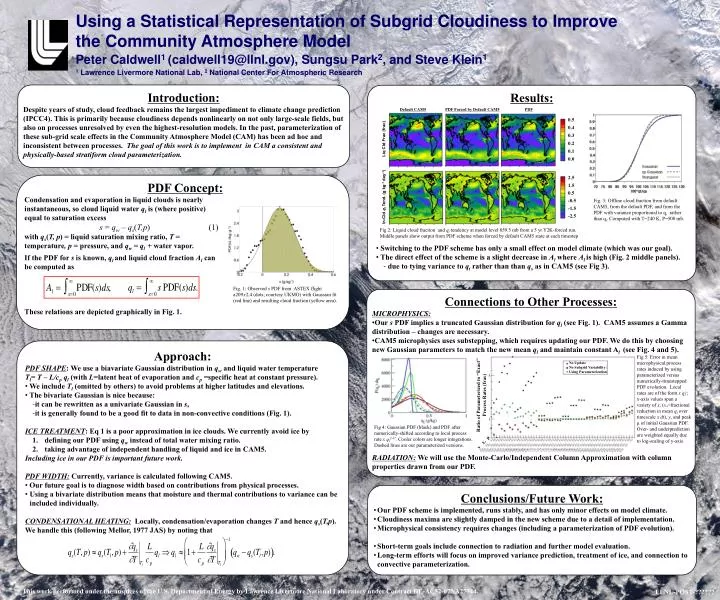
Using a Statistical Representation of Subgrid Cloudiness to Improve the Community Atmosphere Model Peter Caldwell1 (caldwell19@llnl.gov), Sungsu Park2, and Steve Klein1 1 Lawrence Livermore National Lab, 2 National Center For Atmospheric Research Introduction: • Despite years of study, cloud feedback remains the largest impediment to climate change prediction (IPCC4). This is primarily because cloudiness depends nonlinearly on not only large-scale fields, but also on processes unresolved by even the highest-resolution models. In the past, parameterization of these sub-grid scale effects in the Community Atmosphere Model (CAM) has been ad hoc and inconsistent between processes. The goal of this work is to implement in CAM a consistent and physically-based stratiform cloud parameterization. Results: Default CAM5 PDF Forced by Default CAM5 PDF 0.5 0.4 0.3 0.2 0.1 0.0 LiqCldFrac (frac) 2.5 1.5 0.5 -0.5 -1.5 -2.5 PDF Concept: Condensation and evaporation in liquid clouds is nearly instantaneous, so cloud liquid water ql is (where positive) equal to saturation excess s= qw– qs(T,p) (1) • with qs(T, p) = liquid saturation mixing ratio, T = temperature, p= pressure, and qw= ql+ water vapor. If the PDF for s is known, qland liquid cloud fraction Al can be computed as These relations are depicted graphically in Fig. 1. In-Cldql Tend. (g kg-1 day-1) Fig. 3: Offline cloud fraction from default CAM5, from the default PDF, and from the PDF with variance proportional to qsrather than qt. Computed with T=240 K, P=500 mb. Fig 2: Liquid cloud fraction and ql tendency at model level 859.5 mb from a 5 yr Y2K-forced run. Middle panels show output from PDF scheme when forced by default CAM5 state at each timestep • Switching to the PDF scheme has only a small effect on model climate (which was our goal). • The direct effect of the scheme is a slight decrease in Al where Al is high (Fig. 2 middle panels). • due to tying variance to qt rather than than qs as in CAM5 (see Fig 3). Fig. 1: Observed sPDF from ASTEX flight a209.r2.4 (dots; courtesy UKMO) with Gaussian fit (red line) and resulting cloud fraction (yellow area). Connections to Other Processes: • MICROPHYSICS: • Our sPDF implies a truncated Gaussian distribution for ql (see Fig. 1). CAM5 assumes a Gamma distribution – changes are necessary. • CAM5 microphysics uses substepping, which requires updating our PDF. We do this by choosing new Gaussian parameters to match the new mean ql and maintain constant Al (see Fig. 4 and 5). • RADIATION:We will use the Monte-Carlo/Independent Column Approximation with column properties drawn from our PDF. Approach: • PDF SHAPE: We use a biavariate Gaussian distribution in qw and liquid water temperature • Tl= T – L/cpql(with L=latent heat of evaporation and cp=specific heat at constant pressure). • We include Tl(omitted by others) to avoid problems at higher latitudes and elevations. • The bivariate Gaussian is nice because: • it can be rewritten as a univariate Gaussian in s, • it is generally found to be a good fit to data in non-convective conditions (Fig. 1). • ICE TREATMENT: Eq 1 is a poor approximation in ice clouds. We currently avoid ice by • defining our PDF using qw instead of total water mixing ratio. • taking advantage of independent handling of liquid and ice in CAM5. • Including ice in our PDF is important future work. • PDF WIDTH: Currently, variance is calculated following CAM5. • Our future goal is to diagnose width based on contributions from physical processes. • Using a bivariate distribution means that moisture and thermal contributions to variance can beincluded individually. • CONDENSATIONAL HEATING: Locally, condensation/evaporation changes T and hence qs(T,p). We handle this (following Mellor, 1977 JAS) by noting that Fig 5: Error in mean microphysical process rates induced by using parameterized versus numerically-timestepped PDF evolution. Local rates are of the formxqly; x-axis values span a variety of x,(x*=fractional reduction in mean ql over timescale xdt), y, and peak μ of initial Gaussian PDF. Over- and underprediction are weighted equally due to log-scaling of y-axis. No Update No Subgrid Variability Using Parameterization Ratio of Parameterized to “Exact” Process Rates (frac) Fig 4: Gaussian PDF (black) and PDF after numerically-shifted according to local process rate x ql2.47. Cooler colors are longer integrations. Dashed lines are our parameterized versions. yx*μ Conclusions/Future Work: • Our PDF scheme is implemented, runs stably, and has only minor effects on model climate. • Cloudiness maxima are slightly damped in the new scheme due to a detail of implementation. • Microphysical consistency requires changes (including a parameterization of PDF evolution). • Short-term goals include connection to radiation and further model evaluation. • Long-term efforts will focus on improved variance prediction, treatment of ice, and connection to convective parameterization. This work performed under the auspices of the U.S. Department of Energy by Lawrence Livermore National Laboratory under Contract DE-AC52-07NA27344. LLNL-POST-??????