Download
1 / 53
600 likes | 1.18k Views
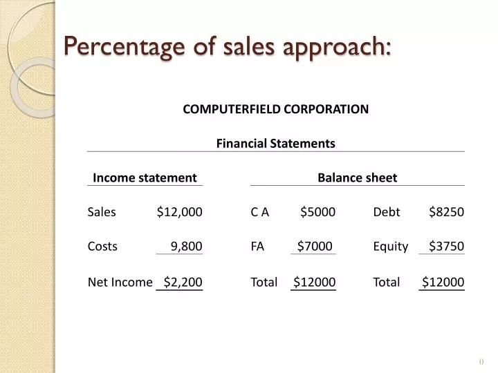
Percentage of sales approach:. EFN and Capacity Usage. Suppose COMPUTERFIELD is operating at 75% capacity: 1. What would be sales at full capacity? (1p) 2. What is the capital intensity ratio at full capacity? (1p)

E N D
EFN and Capacity Usage • Suppose COMPUTERFIELD is operating at 75% capacity: 1. What would be sales at full capacity? (1p) 2. What is the capital intensity ratio at full capacity? (1p) 3. What is EFN at full capacity and Dividend payout ratio is 25%?(ignore accounts payable) (1p)
Q 1:12,000/.75=16,000; Full capacity as % increase16,000/12,000 = 1.33 • Income statement • Sales $12,000 • Costs $9,800 • N I $2,200 • Ret earnings 2,200*.75=1,650 • New ret earnings 1,650*1.33=2,195.5 • There is no indication that any changes took place in % cost for the proforma income statement, we can get the same result by increasing RE or by creating proforma IS
New assets needed • CA • 5000*1.33=6,650 • TA =6,650+7000 • 13,650 • capital intensity ratio at full capacity • =13,650/16,000 =0.8531 • EFN =0 change in TA = 1650 which is less than the retained earnings, we can fully finance internally full capacity operation.
Statistics • Average and std deviation of returns (2p) • Z score for first year return (1p)
16000; 33% increase in sales CA increase 1650capital intensity =.8531
Chapter 13 Return risk and the Security market linehttp://www.quantfinancejobs.com/jobdetails.asp?dbid=&guid=&JobID=9913http://www.quantspot.com/jobs/toronto
Chapter Outline • Expected Returns and Variances of a portfolio • Announcements, Surprises, and Expected Returns • Risk: Systematic and Unsystematic • Diversification and Portfolio Risk • Systematic Risk and Beta • The Security Market Line (SML)
Expected Returns (1) • Expected returns are based on the probabilities of possible outcomes • Expected means average if the process is repeated many times Expected return = return on a risky asset expected in the future
Expected Returns (2) • RA = • RB = • If the risk-free rate = 3.2%, what is the risk premium for each stock?
Variance and Standard Deviation (1) • Unequal probabilities can be used for the entire range of possibilities • Weighted average of squared deviations
Variance and Standard Deviation (2) • Consider the previous example. What is the variance and standard deviation for each stock? • Stock A • Stock B
Portfolios • The risk-return trade-off for a portfolio is measured by the portfolio expected return and standard deviation, just as with individual assets Portfolio = a group of assets held by an investor Portfolio weights = Percentage of a portfolio’s total value in a particular asset
Portfolio Weights • Suppose you have $ 20,000 to invest and you have purchased securities in the following amounts. What are your portfolio weights in each security? • $5,000 of A • $9,000 of B • $5,000 of C • $1,000 of D
Portfolio Expected Returns (1) • The expected return of a portfolio is the weighted average of the expected returns for each asset in the portfolio • You can also find the expected return by finding the portfolio return in each possible state and computing the expected value
Expected Portfolio Returns (2) • Consider the portfolio weights computed previously. If the individual stocks have the following expected returns, what is the expected return for the portfolio? • A: 19.65% • B: 8.96% • C: 9.67% • D: 8.13% • E(RP) =
Portfolio Variance (1) Steps: • Compute the portfolio return for each state:RP = w1R1 + w2R2 + … + wnRn • Compute the expected portfolio return using the same formula as for an individual asset • Compute the portfolio variance and standard deviation using the same formulas as for an individual asset
Portfolio Variance (2) • Consider the following information Invest 60% of your money in Asset A • State Probability A B • Boom .5 70% 10% • Recession .5 -20% 30% • What is the expected return and standard deviation for each asset? • What is the expected return and standard deviation for the portfolio?
Another Way to Calculate Portfolio Variance • Portfolio variance can also be calculated using the following formula: • Correlation is a statistical measure of how 2 assets move in relation to each other • If the correlation between stocks A and B = -1, what is the standard deviation of the portfolio?
Diversification (1) • There are benefits to diversification whenever the correlation between two stocks is less than perfect (p < 1.0) • If two stocks are perfectly positively correlated, then there is simply a risk-return trade-off between the two securities.
Expected vs. Unexpected Returns • Expected return from a stock is the part of return that shareholders in the market predict (expect) • The unexpected return (uncertain, risky part): • At any point in time, the unexpected return can be either positive or negative • Over time, the average of the unexpected component is zero Total return = Expected return + Unexpected return
Announcements and News • Announcements and news contain both an expected component and a surprise component • It is the surprise component that affects a stock’s price and therefore its return Announcement = Expected part + Surprise
Systematic Risk • Risk factors that affect a large number of assets • Also known as non-diversifiable risk or market risk • Examples: changes in GDP, inflation, interest rates, general economic conditions
Unsystematic Risk • Risk factors that affect a limited number of assets • Also known as diversifiable risk and asset-specific risk • Includes such events as labor strikes, shortages.
Returns • Unexpected return = systematic portion + unsystematic portion • Total return can be expressed as follows: Total Return = expected return + systematic portion + unsystematic portion
Effect of Diversification • Portfolio diversification is the investment in several different asset classes or sectors • Diversification is not just holding a lot of assets Principle of diversification = spreading an investment across a number of assets eliminates some, but not all of the risk
The Principle of Diversification • Diversification can substantially reduce the variability of returns without an equivalent reduction in expected returns • Reduction in risk arises because worse than expected returns from one asset are offset by better than expected returns from another • There is a minimum level of risk that cannot be diversified away and that is the systematic portion
Diversifiable (Unsystematic) Risk • The risk that can be eliminated by combining assets into a portfolio • If we hold only one asset, or assets in the same industry, then we are exposing ourselves to risk that we could diversify away • The market will not compensate investors for assuming unnecessary risk
Total Risk • The standard deviation of returns is a measure of total risk • For well diversified portfolios, unsystematic risk is very small • Consequently, the total risk for a diversified portfolio is essentially equivalent to the systematic risk
Systematic Risk Principle • There is a reward for bearing risk • There is no reward for bearing risk unnecessarily • The expected return (and the risk premium) on a risky asset depends only on that asset’s systematic risk since unsystematic risk can be diversified away
Measuring Systematic Risk • Beta (β) is a measure of systematic risk • Interpreting beta: • β = 1 implies the asset has the same systematic risk as the overall market • β < 1 implies the asset has less systematic risk than the overall market • β > 1 implies the asset has more systematic risk than the overall market
Portfolio Betas • Consider the previous example with the following four securities • Security Weight Beta • A .133 3.69 • B .2 0.64 • C .267 1.64 • D .4 1.79 • What is the portfolio beta?
Beta and the Risk Premium • The higher the beta, the greater the risk premium should be • The relationship between the risk premium and beta can be graphically interpreted and allows to estimate the expected return
Consider a portfolio consisting of asset A and a risk-free asset. Expected return on asset A is 20%, it has a beta = 1.6. Risk-free rate = 8%.
Reward-to-Risk Ratio: • The reward-to-risk ratio is the slope of the line illustrated in the previous slide • Slope = (E(RA) – Rf) / (A – 0) • Reward-to-risk ratio = • If an asset has a reward-to-risk ratio = 8? • If an asset has a reward-to-risk ratio = 7?
The Fundamental Result • The reward-to-risk ratio must be the same for all assets in the market • If one asset has twice as much systematic risk as another asset, its risk premium is twice as large
Security Market Line (1) • The security market line (SML) is the representation of market equilibrium • The slope of the SML is the reward-to-risk ratio: (E(RM) – Rf) / M • The beta for the market is always equal to one, the slope can be rewritten Slope = E(RM) – Rf = market risk premium