Download
1 / 25
250 likes | 387 Views
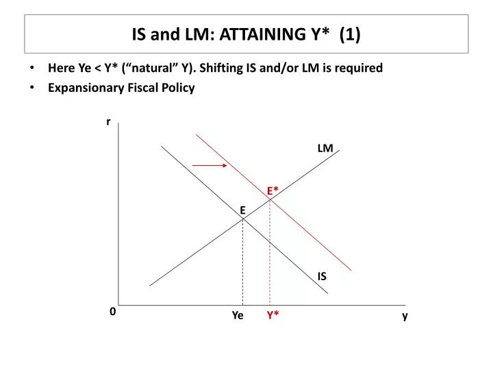
IS and LM: ATTAINING Y* (1). Here Ye < Y* (“natural” Y). Shifting IS and/or LM is required Expansionary Fiscal Policy. r. LM. E*. E. IS. 0. Ye. Y*. y. IS and LM: ATTAINING Y* (2). Here Ye < Y* (“natural” Y). Expansionary Monetary Policy. r. LM. E. E*. IS. 0. Ye. y. Y*.

E N D
IS and LM: ATTAINING Y* (1) • Here Ye < Y* (“natural” Y). Shifting IS and/or LM is required • Expansionary Fiscal Policy r LM E* E IS 0 Ye Y* y
IS and LM: ATTAINING Y* (2) • Here Ye < Y* (“natural” Y). • Expansionary Monetary Policy r LM E E* IS 0 Ye y Y*
FISCAL POLICY EFFECTIVENESS AND “CROWDING OUT” (1) • Here: Steep LM implies low interest-elasticity of Mdand Relatively ineffective fiscal policy (y small) r LM E2 E1 IS2 IS1 0 Y1 Y2 y
FISCAL POLICY EFFECTIVENESS AND “CROWDING OUT” (2) • Here: flat LM implies high interest-elasticity of Md. Relatively effective fiscal policy (y large) r LM E2 E1 IS2 IS1 0 Y1 Y2 y
FISCAL POLICY EFFECTIVENESS AND “CROWDING OUT” (3) • “Crowding out” refers to the fact that a fiscal expansion, with no associated monetary expansion increased Md, increases r, and this reduces Investment and (especially durable goods) Consumption • The less interest-elastic is Md, the more r will have to increase to eliminate excess Money demand • Clearly, if Money is mainly held as a medium of exchange, for which there are few if any substitutes, the less interest-elastic is Md • Also note that all of this applies in a closed-economy context. • Later looking at the open economy we will see that there are differences in how fiscal policy works depending on fixed or flexible exchange rate
MONETARY POLICY EFFECTIVENESS (1) • Ye < Y*: Monetary Expansion • Here steep IS-curve results in small y: why? r LM E1 E2 IS 0 Y1 y Y2
MONETARY POLICY EFFECTIVENESS (2) • Ye < Y*: Monetary Expansion • Here flat IS-curve results in relatively large y: why? r LM E1 E2 IS 0 Y1 y Y2
MONETARY POLICY EFFECTIVENESS (3) • A Monetary expansion operates by excess Ms and lower r, which lead to an increase in real demand (especially Investment) • If real demand is unresponsive (steep IS-curve), then r may fall quite a lot, but y may not increase very much. • The more responsive real demand is to a change in r, the more effective the Monetary expansion • Similarly, the effectiveness of a monetary contraction in curbing demand and y depends on how responsive expenditure is to a change in r • In the open economy, monetary policy may operate in a fundamentally different way: more later
FISCAL MULTIPLIERS IN THE IS-LM MODEL • We have: Y = C + I + G +NX • Now:I = Ia + br,so Ap = Ca + Ia + G + X • Previously: Induced Exp = c(Y t.Y) – zY • Now:Induced Exp = c(Y t.Y) + br – zY • And for a change in Ap we get: Ye = Ap + (Induced Exp) • i.e. Ye = Ap + cY - ctY + br - z Y (1) • No change in Ms Ms = Md = 0 = a Y + f r • and r = a Y/f, and substituting into Eqn (1): • Ye = Ap + cY - ctY – (ab/f)Y - z Y • Ye(1 – c + ct + ab/f – z) = Ap • So Ye/Ap = 1/(1 – c + ct + ab/f – z) NB: (ab/f) > 0 • As f 0, Ye/Ap 0; as f - ; Ye/Ap 1/(1 – c + ct + z) • NB the larger a (dMd/dY) and b (dIp/dr) the smaller Ye/Ap
MONETARY POLICY EFFECTS IN IS-LM • LM shift: Ms = Md = a Y + f r • i.e. fr = Ms a Y • And: r = Ms/f (a/f) Y • Ye = (Induced Exp) (NB: Ap = 0) • i.e. Ye = cY - ctY + br - z Y • and substituting for r : • Y = cY - ctY - z Y (ba/f) Y + (b/f) Ms • Y (1 – c + ct +z +ba/f) = (b/f) Ms • and Y/Ms = (b/f)/ (1 – c + ct +z +ba/f) (NB: b/f > 0) • Note: as b 0, Y/Ms 0 (vertical IS-curve) • Note: as f - , Y/Ms 0 (horizontal LM-curve)
POLICY DISCUSSION (1) • What lessons can we learn from the model in terms of current policy issues? • For Ireland the discussion is largely confined to Fiscal Policy as there is no independent monetary policy. However even with an independent currency an SOE like Ireland would be constrained in terms of policy choices. (more later) • Fiscal policy Government expenditure multipliers are likely to be low because of high marginal tax and import leakages: Significantly < 1 • Tax multipliers are of course negative, but smaller in absolute magnitude, because part of T is reflected in reduced imports and savings • For a small Eurozone member, should there a negative feedback from a fiscal expansion leading to higher interest rates? • Is Irish fiscal policy in a pro-cyclical trap?
POLICY DISCUSSION (2) • See: Gordon pp. 104-105 on Easy Money and Boom and Bust in Housing • The ECB like other Central Banks has a low inflation objective • The general measure used is the CPI or HICP for Eurozone • What if HICP inflation is low, but relatively lax monetary policy leads to rapid increase in asset prices? Should asset prices be part of the ECB’s or Fed’s responsibility? • More particularly should there be action to prevent asset price bubbles? How do you identify bubbles, particularly ex ante? • Part of the problem may have been the downward pressure on the CPI caused by globalisation (entry of China and other Asian economies into trade in a big way): this made tackling the asset bubble more difficult (fear of deflation) • Also the role of big macro imbalances (e.g. USA, China)
POLICY DISCUSSION (3) • In “normal” recessions, individual economies will be a different phases of the cycle, and different policies are warranted. • In 2009-10, we have a severe recession, which is in large measure common to all OECD economies, (sparked off by a common cause: inappropriate monetary policy and regulatory failure, and consequent financial collapse) and policy co-ordination is an issue: • International Fiscal policy co-ordination • International Monetary Policy (later) • Fiscal Policy: • size of individual Eurozone country multipliers • Spillover effects and size of multipliers for co-ordinated fiscal stimulus • Another important issue: Fiscal and Monetary policy operating in combination
MONETARY AND FISCAL POLICY INADEQUATE? • Pure fiscal stimulus: higher r and borrowing costs, etc • Pure monetary expansion: Nominal r 0, y2 still < y* r r LM1 LM LM2 IS IS2 IS1 0 0 y1 y2 y* y y1 y2 y* y
MONETARY AND FISCAL POLICY COMBINED • Severe recession: fiscal stimulus + “quantitative easing” • Longer-run inflationary dangers? r IS1 IS2 LM2 LM1 0 y y1 y*
Caveat • Not Modeled the Open Economy • This will change some of the results significantly
Aside: BALANCED BUDGET MULTIPLIERS (1) • Earlier we derived a multiplier for tax changes in a simple Keynesian model: • Y/ T = – c/(1 – c) • Suppose we have a balanced budget change, i.e. G = T • Multiplier for the expenditure component: Y/G = 1/(1 – c) • The sum of these components = (1– c)/(1 – c) = 1 • Note that this is independent of c and of the size of the component multipliers. • For the IS-LM case, assume G = T and that T, T are exogenous, so that C = Ca + c(Y – T) • and when T changes C = c(Y – T) • Now assume we have G = T
BALANCED BUDGET MULTIPLIERS (2) • For equilibrium: Y = E = G + cY – cT – (ab/f)Y – z Y • i.e. Y (1 – c + z + ab/f) = G – cT = G(1 – c) • so Y/G = (1 – c)/(1 – c + z + ab/f), which is > 0 and < 1 • The intuition behind this is the same: the impact of €1m of G on demand is > than that of €1m of T, as some of the +T comes out of what would have otherwise been saved (and some of the proceeds of a tax cut are saved instead of being spent) • If instead of exogenous T we have T = tY, the result will be similar, but more complicated to derive, because the final change in T is endogenous…..
Some Examples of ISLM in Practice • We apply ISLM to real world historical examples • Kennedy Tax cut • Regan Tax cut • Great Depression • Japan after 1990 • German Unification • US in 1990s • Note these are SR effects because simplistic view of supply side • Also treats economy as being closed
Kennedy Tax Cut • 1964 cut in taxes lead to economic growth • What does IS-LM suggest? • IS shifts up, LM constant • Output rises, interest rate rises • What happened 1964-65? • Regan Tax Cut
The Great Depression • What caused the Great Depression? • Keynes Question • Money shocks or Spending shocks? • Spending • Y down and r down : IS left • why spending down? • Stock Market, Housing, bank failures, federal budget
Monetary Shock • Problem is on the LM • Friedman blames Fed • Should be rise in interest rates • Price Changes
Japan after 1990 • After 1990 Japan’s growth went from spectacular to awful • Shift in IS curve • Output decline (or growth) • Interest decline • Why IS shift? • Share prices and wealth • Credit crunch
German Unification • Blanchard p117 • Fiscal Expansion to pay for redevelopment of east • IS shifts right • Bundesbank fears inflation (see later) • Reduce money supply • LM shifts up • Net effect: • Y up, r up, deficit up • Recession in Europe!
US in 1990s • Think of the effect of contraction of money supply • LM curve shifts up (to left) • Output should fall • R should rise • Price is assumed to be unaffected • See graph : note the price effect