Depth-First and Breadth-First Search

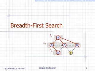
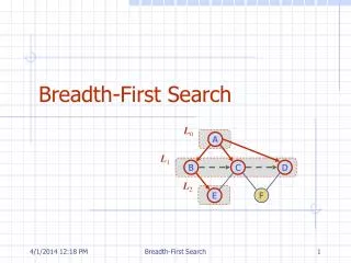
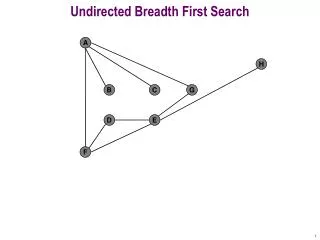
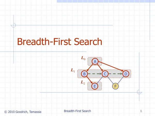
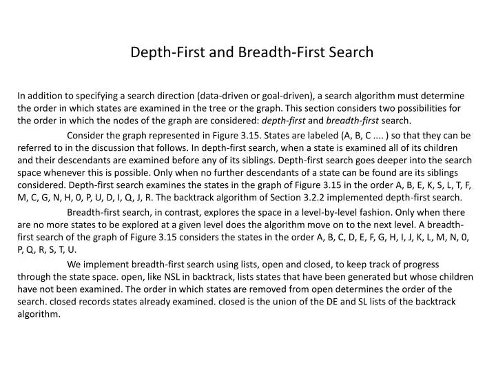
1. Depth-First and Breadth-First Search In addition to specifying a search direction (data-driven or goal-driven), a search algorithm must determine the order in which states are examined in the tree or the graph. This section considers two possibilities for the order in which the nodes of the graph are considered: depth-first and breadth-first search. Consider the graph represented in Figure 3.15. States are labeled (A, B, C .... ) so that they can be referred to in the discussion that follows. In depth-first search, when a state is examined all of its children and their descendants are examined before any of its siblings. Depth-first search goes deeper into the search space whenever this is possible. Only when no further descendants of a state can be found are its siblings considered. Depth-first search examines the states in the graph of Figure 3.15 in the order A, B, E, K, S, L, T, F, M, C, G, N, H, 0, P, U, D, I, Q, J, R. The backtrack algorithm of Section 3.2.2 implemented depth-first search. Breadth-first search, in contrast, explores the space in a level-by-level fashion. Only when there are no more states to be explored at a given level does the algorithm move on to the next level. A breadth-first search of the graph of Figure 3.15 considers the states in the order A, B, C, D, E, F, G, H, I, J, K, L, M, N, 0, P, Q, R, S, T, U. We implement breadth-first search using lists, open and closed, to keep track of progress through the state space. open, like NSL in backtrack, lists states that have been generated but whose children have not been examined. The order in which states are removed from open determines the order of the search. closed records states already examined. closed is the union of the DE and SL lists of the backtrack algorithm.

3. function breadth_first_search; begin open := [Start]; % initialize closed := [ ]; while open ≠ [ ] do % states remain begin remove leftmost state from open, call it X; if X is a goal then return SUCCESS % goal found else begin generate children of X; put X on closed; discard children of X if already on open or closed; % loop check put remaining children on right end of open % queue end end return FAIL % no states left end.

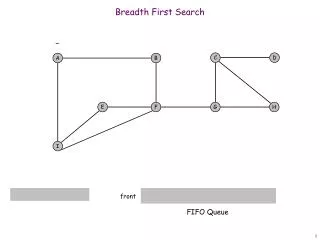
4. Child states are generated by inference rules, legal moves of a game, or other state transition operators. Each iteration produces all children of the state X and adds them to open. Note that open is maintained as a queue, or first-in-first-out (FIFO) data structure. States are added to the right of the list and removed from the left. This biases search toward the states that have been on open the longest, causing the search to be breadth-first. Child states that have already been discovered (already appear on either open or closed) are discarded. If the algorithm terminates because the condition of the "while" loop is no longer satisfied (open = [ ]) then it has searched the entire graph without finding the desired goal: the search has failed. A trace of breadth_first_search on the graph of Figure 3.15 follows. Each successive number, 2,3,4, ... , represents an iteration of the "while" loop. U is the goal state. 1. open = [A]; closed = [] 2. open = [B,C,D]; closed = [A] 3. open = [C,Q,E,F]; closed = [B,A] 4. open = [D,E,F,G,H]; closed = [C,B,A] 5. open = [E.F,G,H,I,J]; closed = [D,C,B,A] 6. Open = [F,G,H,I,J,K,L]: closed = [E,D.C,B,A] 7. open = [G,H,I,J,K,L,M] (as L is already on open); closed = [F,E,D,C,B,A] 8. open = [H,I,J,K,L,M,N]: closed = [G,F,E,D,C,B,A] 9. and so on until either U is found or open = [ ] Figure 3.16 illustrates the graph of Figure 3.15 after six iterations of breadth-first-search. The states on open and closed are highlighted. States not shaded have not been discovered by the algorithm. Note that open records the states on the "frontier" of the search at any stage and that closed records states already visited.

6. Because breadth-first-search considers every node at each level of the graph before going deeper into the space, all states are first reached along the shortest path from the start state. Breadth-first-search is therefore guaranteed to find the shortest path from the start state to the goal. Furthermore, because all states are first found along the shortest path, any states encountered a second time are found along a path of equal or greater length. Because there isno chance that duplicate states were found along a better path, the algorithm simply discards any duplicate states. It is often useful to keep other information on open and closed besides the names of the states.For example, note that breadth_first_search does not maintain a list of states on the current path to a goal as backtrack did on the list SL; all visited states are kept on closed. If the path is required for a solution, it can be returned by the algorithm. This can be done by storing ancestor information along with each state. A state may be saved along with a record of its parent state, i.e., as a (state, parent) pair. If this is done in the search of Figure 3.15, the contents of open and closed at the fourth iteration would be: open = [(D,A), (E.B), (F,B), (G,C), (H,C)]; closed = [(C,A), (B,A), (A,nil)] The path (A, B, F) that led from A to F could easily be constructed from this information. When a goal is found, the algorithm may construct the solution path by tracing back along parents from the goal to the start state. Note that state A has a parent of nil, indicating that it is a start state; this stops reconstruction of the path. Because breadth-first-search finds each state along the shortest path and retains the first version of each state, this is the shortest path from a start to a goal. Figure 3.17 shows the states removed from open and examined in a breadth-first-search of the graph of the 8-puzzle. As before, arcs correspond to moves of the blank up, to the right, down, and to the left. The number next to each state indicates the order in which it was removed from open. States left on open when the algorithm halted are not shown. Next, we create a depth-first search algorithm, a simplification of the backtrack algorithm already presented in Section 3.2.3. In this algorithm, the descendant states are added and removed from the left end of open: open is maintained as a stack, or last-in-first-out (LIFO), structure. The organization of open as a stack directs search toward the most recently generated states, producing a depth-first search order:

8. begin open := [Start]; % initialize closed := [ ]; while open ≠ [ ] do % states remain begin remove leftmost state from open, call it X; if X is a goal then return SUCCESS % goal found else begin generate children of X; put X on closed; discard children of X if already on open or closed; % loop check put remaining children on left end of open % queue end end; return FAIL % no states left end. A trace of depth-first-search on the graph of Figure 3.15 appears below. Each successive iteration of the "while" loop is indicated by a single line (2, 3, 4, ... ). The initial states of open and closed are given on line 1. Assume U is the goal state. 1. open = [A]; closed= [] 2. open= [B,C,D]; closed = [A] 3. open =, [E,F,C,D]; closed = [B,A]

9. 4. open = [K,L,F,C,D]; closed = [E,B,A] S. open [S,L,F,C,D]; closed = [K,E,B,A] 6. open = [L,F,C,D]; closed = [S,K,E,B,A] 7. open", [T,F,C,D]; closed = [L,S,K,E,B,A] 8. open = [F,C,D]; closed = [T,L,S,K,E,B,A] 9. open = [M,C,D]; (as L is already on closed); closed = [F,T,L,S,K,E,B,A] 10. open = [C,D]; closed = [M,F,T,L,S,K,E,B,A] II. open = [G,H,D]; closed = [C,M,F,T,L,S,K,E,B,A] and so on until either U is discovered or open = [ ]. As with breadth_first_search, open lists all states discovered but not yet evaluated (the current "frontier" of the search), and closed records states already considered. Figure 3.18 shows the graph of Figure 3.15 at the sixth iteration of the depth-first-search. The contents of open and closed are highlighted. As with breadth-first-search, the algorithm could store a record of the parent along with each state, allowing the algorithm to reconstruct the path that led from the start state to a goal. Unlike breadth-first search, a depth-first search is not guaranteed to find the shortest path to a state the first time that state is encountered. Later in the search, a different path may be found to any state. If path length matters in a problem solver, when the algorithm encounters a duplicate state, the algorithm should save the version reached along the shortest path. This could be done by storing each state as a triple: (state, parent, length_of_path). When children are generated, the value of the path length is simply incremented by one and saved with the child. If a child is reached along multiple paths, this information can be used to retain the best version. This is treated in more detail in the discussion of algorithm A in Chapter 4. Note that retaining the best version of a state in a simple depth-first search does not guarantee that a goal will be reached along the shortest path. Figure 3.19 gives a depth-first search of the 8-puzzle. As noted previously, the space is generated by the four "move blank" rules (up, down, left, and right). The numbers next to the states indicate the order in which they were considered, i.e., removed from open. States left on open when the goal is found are not shown. A depth bound of 5 was imposed on this search to keep it from getting lost deep in the space.

12. As with choosing between data- and goal-driven search for evaluating a graph, the choice of depth-first or breadth-first search depends on the specific problem being solved. Significant features include the importance of finding the shortest path to a goal, the branching factor of the space, the available compute time and space resources, the average length of paths to a goal node, and whether we want all solutions or only the first solution. In making these decisions, there are advantages and disadvantages for each approach. Breadth-First Because it always examines all the nodes at level n before proceeding to level n + 1, breadth-first search always finds the shortest path to a goal node. In a problem where it is known that a simple solution exists, this solution will be found. Unfortunately, if there is a bad branching factor, i.e., states have a high average number of descendants, the combinatorial explosion may prevent the algorithm from finding a solution using the available space. This is due to the fact that all unexpanded nodes for each level of the search must be kept on open. For deep searches, or state spaces with a high branching factor, this can become quite cumbersome. The space utilization of breadth-first search, measured in terms of the number of states on open, is an exponential function of the length of the path at any time. If each state has an average of B children, the number of states on a given level is B times the number of states on the previous level. This gives Bnstates on level n. Breadth-first search would place all of these on open when it begins examining level n. This can be prohibitive if solution paths are long. Depth-First Depth-firstsearch gets quickly into a deep search space. If it is known that the solution path will be long, depth-first search will not waste lime searching a large number of "shallow" states in the graph. On the other hand, depth-first search can get "lost"" deep in a graph, missing shorter paths to a goal or even becoming stuck in an infinitely long path that does not lead to a goal. Depth-first search is much more efficient for search spaces with many branches because it does not have to keep all the nodes at a given level on the open list.

13. The space usage of depth-first search is a linear function of the length of the path. At each level, open retains only the children of a single state. If a graph has an average of 8 children per state, this requires a total space usage of B x n states to go n levels deep into the space. The best answer to the "depth-first versus breadth-first" issue is to examine the problem space carefully and consult experts in the area. In chess, for example, breadth-first search simply is not possible. In simpler games, breadth-first search not only may be possible but also may be the only way to avoid losing. Depth-First Search with Iterative Deepening A nice compromise on these trade-offs is to use a depth bound on depth-first search. The depth bound forces a failure on a search path once it gets below a certain level. This causes a breadth-like sweep of the search space at that depth level. When it is known that a solution lies within a certain depth or when time constraints, such as those that occur in an extremely large space like chess, limit the number of states that can be considered; then a depth-first search with a depth bound may be most appropriate. Figure 3.19 showed a depth-first search of the 8-puzzle in which a depth bound of 5 caused the sweep across the space at that depth. This insight leads to a search algorithm that remedies many of the drawbacks of both depth-first and breadth-first search. Depth-first iterative deepening (Korf 1987) performs a depth-first search of the space with a depth bound of I. lf it fails to find a goal, it performs another depth-first search with a depth bound of 2. This continues, increasing the depth bound by one at each iteration. At each iteration, the algorithm performs a complete depth-first search to the current depth bound. No information about the state space is retained between iterations.

14. Because the algorithm searches the space in a level-by-level fashion, it is guaranteed to find a shortest path to a goal. Because it does only depth-first search at each iteration, the space usage at any level n is B x n, where B is the average number of children of a node. Interestingly, although it seems as if depth-first iterative deepening would be much less time efficient than either depth-first or breadth-first-search, its time complexity is actually of the same order of magnitude as either of these: 0(Bn). An intuitive explanation for this seeming paradox is given by Korf (1987): Since the number of nodes in a given level of the tree grows exponentially with depth, almost all the time is spent in the deepest level, even though shallower levels are generated an arithmetically increasing number of times. Unfortunately, all the search strategies discussed in this chapter--depth-first, breadth-first, and depth-first iterative deepening-may be shown to have worst-case exponential time complexity. This is true for all uninformed search algorithms. The only approaches to search that reduce this complexity employ heuristics to guide search. Best-first search is a search algorithm that is similar to the algorithms for depth- and breadth-first search just presented. However, best-first search orders the states on the open list, the current fringe of the search, according to some measure of their heuristic merit. At each iteration, it considers neither the deepest nor the shallowest but the "best" state. Best-first search is the main topic of Chapter 4.