Download
1 / 15
150 likes | 218 Views
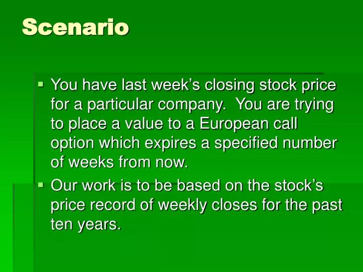
Scenario. You have last week’s closing stock price for a particular company. You are trying to place a value to a European call option which expires a specified number of weeks from now. Our work is to be based on the stock’s price record of weekly closes for the past ten years.

E N D
Scenario • You have last week’s closing stock price for a particular company. You are trying to place a value to a European call option which expires a specified number of weeks from now. • Our work is to be based on the stock’s price record of weekly closes for the past ten years.
Data & Notation • The data set is a ten-year history of weekly closing prices for this stock. • Notation and variables:PV=present value of the European call optionFV=future value of the European call option R=ratio of future to present values Rm=average value of all weekly ratios of closing prices rrf=risk-free rate Rrf=the ratio of future to present values of an investment growing at the risk-free rate Rnorm=the normalized ratios
Goal • The goal is to use all available information to compute the expected value of the price of the option, E(PV). • We do this by first simulating the growth of the stock during the option’s period. • Comparing this value to the strike price, we can estimate the price of the option at the expiration date, FV. • Using the compound interest formula in conjunction with the risk-free rate, we can calculate the price of the option at the start of the period. • After MANY simulations, we may consider this a random sample, take the average of the outcomes, and claim this estimates E(PV).
Organizing Data • 520 ratios + chaotic ordering to values = Reason to create histogram!! • The histogram of ratios is converted to relative frequencies (and when these percentages are divided by the bin width, the graph represents a p.d.f.) • However, the mean of the ratios is higher or lower than Rrf, so we’d like to normalize our ratios.
Normalizing • Normalizing is simply a means by which to standardize our results. • For example, consider two possible savings accounts. Account A compounds interest quarterly at a rate of 4%. Account B compounds interest monthly at a rate of 3.9%. Which account is more likely to acrue more interest?
Normalizing • In order to compare, we need to standardize both accounts—bring both to some equal grounds of comparison. • Normalizing, in this case, involves calculating the annual yield for each account.
Normalizing • In our Project, we need to eliminate the inherent growth rate for a particular stock. This growth rate is embedded in our Rm. To normalize, we need to shift this average, so that our histogram is centered at Rrf. • Rnorm = R – (Rm – Rrf)
Organizing Data • Our p.d.f. is giving us probabilities that a ratio occurs within a certain range. • Rnorm can take on an infinite number of values, therefore it must be a continuous random variable. It is therefore appropriate to use a p.d.f. to describe the distribution of normalized ratios.
Simulation • By randomly choosing n normalized ratios using Excel, where n is the number of weeks before the option expires, we may take the product of these ratios along with the stock’s starting price for this period. This gives us an approximation of the value of the stock at the expiration date.
Simulation • If the stock price is greater than the strike price, specified in the option, then the option is in-the-money, and the option will have the value of stock price – strike price = FV • If the stock price is less than the strike price, then the option is out-of-the-money, and the option is worthless, i.e. FV = 0.
PV • Once a value for FV is known, one can use the assumption that all investments grow at the risk-free rate, and can therefore solve for PV: Here, t is equal to the number of weeks specified in the option, divided by the number of weeks in a year (52).
E(PV) • After running 5000 simulations, we may average all 5000 values of PV to approximate E(PV). • If we do this 40 times, and average these 40 values, what would we expect?
What you should include • Background on company • Summary of 10 year history • Ratio histogram (can leave as relative frequencies) • Normalized ratios (in p.d.f. form) • Explanation of simulation • Results of simulation • Conclusion • Further analysis
Further analysis • Anyone can follow the book’s example and come up with an expected value. But do they really understand what is going on? • The further analysis is a chance for you to show me that you understand what this project is about, and that you understand the tools you are using
Further analysis • No presentation/paper will get an A without including further analysis. • The analysis must be done in a plausible way • Changing the history of the stock is not likely. That has already happened, and cannot change.