Download

1 / 58
580 likes | 716 Views
A Look at Climate Prediction Center’s Products and Services. Ed O’Lenic NOAA-NWS-Climate Prediction Center Camp Springs, Maryland ed.olenic@noaa.gov 301-763-8000, ext 7528 Eastern Region Climate Services Workshop Raliegh, North Carolina September 17, 2003. Objectives.

E N D
A Look at Climate Prediction Center’s Products and Services Ed O’Lenic NOAA-NWS-Climate Prediction Center Camp Springs, Maryland ed.olenic@noaa.gov 301-763-8000, ext 7528 Eastern Region Climate Services Workshop Raliegh, North Carolina September 17, 2003
Objectives • CPC products and terms • CPC’s web site • MJO & tropical convection - hope • Outlooks • Verification
Climate Versus Weather Top Graph: Observed daily average Temperature (T), May 2000-April 2001 (jagged curve, an example of “weather”), and 30-year average (1971-2000) of daily average T (also called the “normal”, (smooth curve) the standard definition of “climate”) at Albany, New York. Note the large day-to-day variability indicated by the red (above-normal) and blue (below normal) daily T events. Bottom Graph: Result of subtracting the normal from the daily average T in the top graph and then performing a 31- day running average. Note the expanded scale on the lower graph. The extended periods of above and below normal 31-day average T are, examples of short-term climate variability. Green line is the average of the departures over May 2000-April 2001.
CPC Data-to-Product Process Schematic REAL-TIME OBS DYNAMICAL MODEL ENSEMBLES HISTORICAL OBSERV-ATIONS CLIMO STATISTICAL MODELS MONITORING - PREDICTION TOOLS, WEB PAGES FORECASTS, EXPERT ASSESSMENTS, MONITORING PRODUCTS AWIPS, PRINTED PUBLICATIONS, WEB PAGES/AUTOMATED PRODUCTS AND DATABASES USER FEEDBACK VIA CSD
Some Definitions • Climate: Average of weather over days, weeks, months, years • Climate Prediction: Concerned with averages and variability, rather than weather. • Climatology: Average over a long time relative to features being studied (BORING) • 3-class system: Divide the climatology into highest, lowest and middle thirds. • Lead time: Time between the issuance of a forecast and when it becomes valid. • 6-10 day forecast: 5-day mean forecast at lead 5 days. • 8-14 day forecast: 7-day mean forecast at lead 7 days. • 0.5 month outlook: ½ month lead forecast of seasonal mean T, P • Probability = P(A) = (# possible events (H)) / (total # possible outcomes (H+T)) • Probability anomaly: probability of an event – climatological probability of an event. • Total probability: probability anomaly + climatological probability • Probability distribution: Graph where the area under the curve=prob. of an event. • Extreme event: An event in the upper-, or lower-most part of a probability dist. • Southern Oscillation: A back and forth pressure variation with opposite sign between the eastern (Tahiti) and western (Darwin) portions of the tropical Pacific. • ENSO: El Nino/Southern Oscillation, made up of El Nino (warm) and La Nina (cold) • ENSO-Neutral: Usually refers to years which are neither El Nino nor La Nina • Trend: most recent 10(15) year means of observed T(P) minus the 30-yr climatology • Maritime Continent: Indonesia and surrounding region, a focus of tropical convection • MJO: Madden-Julian Oscillation, a wave #1 tropical disturbance with dry and wet phases which moves from west-to-east around the global tropics in 30-60 days.
Total SST7-day mean centered on 03 September, 2003SSTa Warm Pool nino 3.4 Cold Tongue
The U.S. Hazards Assessment page is a comprehensive source of up-to- date information on the status of the Global climate. The left column is intended to let you self-brief, and is used by Hazards briefers to prepare and brief the product. Climate HighlightsUS Hazards Assessment
Climate Highlights – ENSO Diagnostic Discussionhttp://www.cpc.ncep.noaa.gov/products/analysis_monitoring/enso_advisory/index.html
Outlooks – Products http://www.cpc.ncep.noaa.gov/products/predictions Outlook Products link
S/N is larger for Seasonal than Monthly. Monthly Outlook
0.5 mo lead seasonal T, P outlook Outlooks combine long-term trends, soil-moisture effects, model forecasts with typical ENSO cycle impacts, when appropriate.
Diurnal Cycle of Convection Can Lead to Large Time and Space Scale Phenomena
Why the MJO is important • Intimately related to active/break cycles of the Australian and Asian Monsoons • Offers potential to provide extended predictability up to 15-20 days in tropics • Affects weather (predictably?) over the western US and elsewhere • Associated westerly wind events generate Tropical Pacific ocean Kelvin waves which may significantly modify the evolution and amplitude of El Nino (e.g. 1997, 1991) • Large inter-annual variability in the activity of the MJO has implications for the predictability of the coupled ocean-atmosphere system
MJO Activity and Inter-annual SST 1 season lag correlation = 0.65 • West Pacific SST in Fall versus MJO Activity in Winter • Foundation for link with ENSO? • 95% level assuming zero correlation and 22 dof is 0.43 MJO ACTIVITY West Pacific SST
MJOs and 1991-92 El Nino: Late Onset Zonal Wind Anoms SST Anoms 20C Depth Anoms Nov 90 1 1 2 Mar 91 2 3 Sep 91 3
Annual Mean Precipitation Errors in HadAM3:Sensitivity to Horizontal Resolution (Neale and Slingo, 2003: J. Clim., 16, 834-838)
HadAM3 Sensitivity Experiments: Impact of removing the islands of the Maritime Continent(Neale and Slingo, 2003: J. Clim., 16, 834-838) • Land grid-points removed and replaced by ocean grid-points. • Increased moisture availability from the sea surface leads to enhanced convection and partial correction of the model dry bias. • Note also corrections to model’s wet bias in adjacent areas.
Global Impacts of Improved Maritime Continent Heat SourceDJF: 500hPa height (m) and Surface Temperature (K) • Potential improvements in the Maritime Continent heat source can have significant remote effects. • Related to the generation of Rossby waves by the enhanced divergent outflow from the Maritime Continent heat source. • Substantially reduces model systematic error over the extra-tropics of the winter hemisphere. • Emphasizes the importance of considering the global context of model systematic error in which biases in the tropics may be a key factor.
Forecast Maps and Bulletins • Each month, on the Thursday between the 15th 21st, CPC issues a set of 13 seasonal outlooks. • There are two maps for each of the 13 leads, one for temperature and one for precipitation for a total of 26 maps. • Each outlook covers a 3-month “season”, and each forecast overlaps the next and prior season by 2 months. • Bulletins include: the prognostic discussion for the seasonal outlook over North America, and, for Hawaii. • The monthly outlook is issued at the same time as the seasonal outlook. It consists of a temperature and precipitation outlook for a single lead, 0.5 months, and the monthly bulletin. • All maps are sent to AWIPS, Family of Services and internet.
Statistical Prediction Tools • Multiple Linear Regression: - Predicts a single variable from historical and recent observations of two or more predictors. • Canonical Correlation Analysis (CCA): • Uses recent and historical observations of Northern Hemisphere circulation (Z), global sea surface temperature (SST), US surface T (Tus) to create a set of 5 or 6 EOFs of predictors and predictands. • Looks at cross-correlations between time series of predictors and predictands. • Predicts temporal and spatial patterns from patterns.
Statistical Prediction Tools • Constructed Analogs (CA) • Uses recent observations (base) of a single variable and historical observations, to construct a weighted mean of all prior years which best explains the base data. Assumes the evolution to subsequent seasons is also best explained by the weights used to construct the analog to the base. • Optimal Climate Normals (OCN) • Uses the difference between the most recent 10 (15) years of temperature (precipitation) observations and the 30-year climatology (i.e., the trend) for a given season as the prediction for future occurrences of that season.
Trend (10-yr mean-minus-30-yr mean) Temperature for Alaska and CONUSLoop shows 3-month mean T anomalies expressed as tenths of standard deviations.JAS, ASO, SON, …, MJJ, JJA
http://www.cpc.ncep.noaa.gov/products/predictions/90day/tools/briefing/index.pri.htmlhttp://www.cpc.ncep.noaa.gov/products/predictions/90day/tools/briefing/index.pri.html
NCEP AGCM Forecasts for DJF 2000-01, 2001-02, and 2002-03 Global and NOAM T Fcst SST Forcing 2000-01 2001-02 2002-03
OCN CCA CCA, OCN, CMP, OFF T Tools DJF2003 CMP OFF
PROBABILITY OF EXCEEDANCE ~ THE SHIFT IN THE CENTER OF THE DISTRIBUTION IMPLIED BY THE FORECAST
Verification • CPC official forecasts and tools are continuously verified • Verification statistics are made available to forecasters • Categorical verifications – blunt instrument, understandable • Probabilistic verifications – much more informative, highlight need for calibration
Heidke Skill Score s = ((c-e)/(t-e))*100 c = # stations correct e = # stations expected correct t = # stations in total
Categorical Skill Scores of Seasonal Forecasts0.5 Month-Lead Temperature
Categorical Skill Scores of Seasonal Forecasts0.5 Month-Lead Precipitation