Download
1 / 60
600 likes | 777 Views
Retrieval of Visual Content . Images comprise the vast majority of data in many application domains Remote sensing (NASA, 1 terabyte per day) Astronomy Geographic Information Systems (GIS) Medicine (CT, MRI, etc.) Criminal investigation Trademark authentication.

E N D
Retrieval of Visual Content • Images comprise the vast majority of data in many application domains • Remote sensing (NASA, 1 terabyte per day) • Astronomy • Geographic Information Systems (GIS) • Medicine (CT, MRI, etc.) • Criminal investigation • Trademark authentication Visual Content
Images in Multimedia Systems • Images co-exist with other types of data in Multimedia Documents • text • attribute • video • sound Visual Content
Content-Based Image Retrieval • Descriptions of image content are extracted and stored • Manually: mainly text descriptions • Difficult • Subjective • Automatically: features from content • Computationally expensive • Inexact • Domain specific Visual Content
System Architecture Visual Content
Design Issues • Feature Extraction (functions) • Feature Selection • Organization of stored information, file structures, indexing • Search and retrieval strategies • Sequential / Indexed search / Query refinement • Query language: conditional / example queries • User interface design Visual Content
Image Descriptions • Subjective interpretation of content: means different things to different people • Different features for different applications • Colour is important of out-door image but not for X-rays, CT, MRI etc. • Motion features are sometimes important (ultrasound) • Different systems for different applications Visual Content
Levels Representation • Low at pixel level (e.g., intensities, colors) • Intermediate atregion level (e.g., region, shape, motion features, motion) • High – Semantic human interpretations (e.g., a class per object or image or domain concepts such as diagnosis …) Visual Content
Conflicting issues • Dependence on image content, computational overhead and uncertainty increases from low to high level • Selection depends on application, image type, user requirements, query types Visual Content
Reliability Criteria • Uniqueness • Proportionality of variation • Robustness against noise • Invariance under translation, rotation, scaling • Computationally efficient • Content at various level of detail Visual Content
Generic Features • Feature vectors of • intensity / color • texture • spatial relationships • motion • combinations of the above • Two kinds of features • global: computed for the entire image • local: computed for objects or image parts Visual Content
RGB Color Space • Popular hardware oriented scheme • Colors form a unit cube • r = R/(R+G+B) • g = G/(R+G+B) • b = B/(R+G+B) • RGB is good for acquisition and display but not for the perception of colors Visual Content
Munsell Color Space • Color in cylindrical coordinates • Brightness: vertical axis • Hue: angular displacement • Saturation: cylindrical radius Visual Content
Color Definitions • Brightness: intensity of color, average intensity over all wavelengths • Hue: proportional to the average wavelength of the color percept • Saturation: amount of white, highly saturated colors have no white • deep red has S=1 • pinks have S=0 Visual Content
HSV Color Space • Value • Hue • Saturation • H = undefined for S = 0 • H = 360 – H if B/V > G/V Visual Content
Color in Retrievals • Color Histograms are very common • Simple to compute and compare • For the entire image or for image parts • 3D histogram on RGB or HSV space (224 bins!) • 1D histogram over the 3 primaries (256 bins) • Use HSV histograms: changes in lighting and viewing angles may cause major variations in RGB histograms • Invariant under translation, rotation, viewing angle and scaling Visual Content
1D histogram A.Del Bimbo 99 Visual Content
Histogram Comparison • Histogram intersection • Q, I: histograms of a query and database image • N: histogram bins • 3D (RGB, HSV) intersection is defined accordingly A.Del Bimbo 99 normalized intersection Visual Content
Reducing Complexity • Reduce number of histogram bins • Transform RGB histogram to (rg,by,wb) • rg = R – G, by = 2B – R – G, wb = R + G + B • Intensity wb is more coarsely sampled than rg,by • wb (8 sections), rg, by (16 sections) • The resulting histogram has 2048 bins • Reduced sensitivity to variations of intensity Visual Content
Reducing Complexity (cont,d) • Clustering detects the K most prominent colors (e.g., K-means) • Histogram with K bins (e.g., K=64 or 256) • Each bin is the normalized count of pixels in the cluster Visual Content
Reducing Complexity (cont,d) • Recognize that only a small number of bins capture the majority of pixels • Threshold to take only the large bins • Small bins are likely to be noisy bins thus distorting the intersection • Does not degrade the performance Visual Content
Distance Function • Certain pairs of bins correspond to perceptually similar colors • In intersection all bins are compared independently of each other • Define new Distance function: • A=(aij) represents bin proximity • aij based on proximity in the L*u*v space Visual Content
L*u*v color space A.Del Bimbo 99 Visual Content
Color Indexing • Color (feature) vector: histogram • Problems: • K is large (K=64 or 256) • Quadratic complexity of matching • SAMs assume independent attributes • Solution: GEMINI • Map to low dimensionality feature space • Lower bound distance: Df(I,Q) <= D(I,Q) Visual Content
Definition of Df(I,Q) • Take some average color value on color space (e.g., R,G,B) • average color of image: (Ravg,Gavg,Bavg)= • and Visual Content
GEMINI Approach • Indexing in the 3D color space • Df< D(I,Q): see QBIC paper for proof • Map query Q to the same 3D space • Search the feature space • Clean-up answer set to eliminate false drops Visual Content
Texture • Repeative patterns of local variations of intensity • Structural: identify placement rules of structural primitives • the less effective approach • Statistical: characterize spatial distribution of intensity in terms of measurements • Haralick, Tamura features etc. Visual Content
Texture Examples Ballard and Brown 84 Visual Content
Structural Texture Ballard and Brown 84 Visual Content
Statistical Texture Ballard and Brown 84 Visual Content
Haralick Features [Haralick 73] • Set of 4 features characterizing the intensity transitions of neighboring pixels in various directions using • Gray-Tone Spatial-Dependence (GTSD) arrays • One GTSD for each pixel neighborhood • Neighborhood: pixels in direction θ and distance d Visual Content
GTSD Array Pd,θ[i,j] • Counts pixel pairs in distance d having gray levels i, j in directionθ • One GTSD forθ=(00, 450,900, 1350)and d=(1,2,..) • Intensity in range [0,k-1]: Pd,θ[i,j] is a k x k matrix P[i,j] d = 1 0 i 1 1 j 16 2 0 1 2 Visual Content
Computing Pd,θ[i,j] • Count all pairs of pixels in which the first pixel has value i and its matching pair displaced by d=1 in θ = 450or 1350 direction has value j • Enter this count in the (i,j) position of Pd,θ[i,j] • E.g., there are 3 pairs [2,1], then P[2,1] = 3 • Pd,θ[i,j] is not symmetric: Pd,θ[i,j] < > Pd,θ[j,i] • NormalizePd,θ[i,j] by the total number of pairs • Pd,θ[i,j]: probability mass function Visual Content
Texture Features • Angular Second Moment (ASM): • Small values for non homogeneous regions • Contrast: • Large values for many large transitions or for many transitions Visual Content
Texture Features (cont,d) • Correlation: Frequency of intensity transitions Visual Content
Texture Features (cont,d) • Entropy: • Highvalues for uniform p[i,j] i.e., no preferred gray-level (no texture) • A vector for each Tθ,d=(f1,f2,f3,f4) or • A vector for every θ, d taking all Tθ,din a sequence • Correlated features: apply K-L to de-correlate and to reduce dimensionality Visual Content
Shape • Assume that objects are extracted • Requires image segmentation • Difficult problem • Criteria for reliable shape recognition • Uniqueness of representation • Robustness against noise and distortion • Proportionality of variation • Invariance under scale, rotation and translation • Efficiency of computation • Occlusion: handle partially visible shapes Visual Content
Shape Matching Methods • Two categories of methods based on: • Regions: represent and match properties of regions • Contours: represent and match properties of boundaries • Techniques: local/global, model based, fuzzy, statistical, neural networks Visual Content
Input/Output • For any two shapes and compute: • Their distance • The correspondences between similar parts Petrakis 02 Visual Content
R Moment Invariants • An object is represented by its binary image • A set of 7 features can be defined based on central moments Visual Content
Central Moments [Hu 62] • Invariant to translation and rotation • Use ηpq=μpq/μγ00where γ=(p+q)/2 + 1 for p+q=2,3… instead of μ’s in the above formulas to achieve scale invariance Visual Content
More Shape Methods • Moments can also be defined on the closed bounding contours of objects [Gupta and Shinath 87] • Moments can also be defined for open curves [Koch and Kashyap 89] • Methods based on the Fourier Transform of the bounding contour have also been used [Wallace and Wintz 80, Rauber and Steiger 92] • More efficient methods has also been proposed [Petrakis, Diplaros and Milios 2002]. Examines many of the above methods based on Fourier and Moments and shows many experiments and comparisons Visual Content
Spatial Relationships • Find images showing similar objects in similar spatial relationships • find X-rays similar to Smith’s examination • find images showing a tree close to a house • one of the two images may contain extra objects I Q Petrakis02 Visual Content
Methods • Two main categories of methods • Spatial projections (2D strings and variants like 2D C strings, Expanded 2D strings etc). • Attributed Relational Graphs (ARGs) • Image distance is defined accordingly • Editing distance on ARGs • 2D string matching Visual Content
Image Segmentation • All methods assume segmented images • image are segmented manually or semi-manually • image segmentation is a difficult problem Petrakis02 Visual Content
Image Features • Individual objects: 5-dimensional vectors • Size: number of pixels in a region • Perimeter: length of bounding contour • Roundness: ratio of smallest/largest second moment • orientation: angle with x direction (sin,cos) • Spatial Relationships: 4-dimensional vectors • Position: inside or outside • Distance: minimum distance of contours • Orientation: angle with x (sin,cos) of c.g.’s Visual Content
Attributes Relational Graphs (ARGs) • Objects are represented by nodes • Relationships are represented by arcs • Nodes and arcs are labeled by feature vectors • Matching: ARG editing distance, Hungarian [Petrakis 02] Petrakis02 Visual Content
ARG Editing Distance • Matching: sequence of edit operations that transform a query Q to an image I • Edit operation: node or arc insertion, deletion or substitution • F combines the costs of edit operations • f is the cost of an edit operation defined as a vector distance Visual Content
Matching Algorithm [Messmer95] • Find the sequence of edit operations that yield the minimum total cost • Formulated as tree search problem • Expand all possible matching sequences • Branch and bound • Tree node: matching of ARG node • Tree arc: matching of ARG edges • Subtree: matching of subgraphs of Q, I Visual Content
Query Q Model I Visual Content
Hungarian Method [Petrakis 02] • Matching: assignment problem • The relationships are ignored • F: cost of a mapping • C(i,F(i)): vector distance Visual Content