Download
1 / 33
330 likes | 422 Views
Predicting the In-System Performance of the CMS Tracker Analog Readout Optical Links. Stefanos Dris CERN & Imperial College, London. Introduction. Introduction The Tracker Optical Links Simulation Specifications Results Conclusions.

E N D
Predicting the In-System Performance of the CMS Tracker Analog Readout Optical Links Stefanos Dris CERN & Imperial College, London
Introduction Introduction The Tracker Optical Links Simulation Specifications Results Conclusions • 10 million channels in the CMS Tracker read out by ~40 000 analog optical links. • Electronic, optoelectronic, and optical components making up the readout links will vary in gain. • What spread in gain and dynamic range from link to link can we expect in the final system as a result? • Will system specifications be met? • We are now in a position to find out by simulation based on real production test data.
Analog Readout Optical Links Introduction The Tracker Optical Links Simulation Specifications Results Conclusions
Simulation Simulation: LLD Data Introduction The Tracker Optical Links Simulation Specifications Results Conclusions • LLD has four gain settings, allowing a certain amount of gain equalization of the optical links in the final system.
Simulation Simulation: Laser Tx Data Introduction The Tracker Optical Links Simulation Specifications Results Conclusions
Simulation Simulation: AOH Data Introduction The Tracker Optical Links Simulation Specifications Results Conclusions • Calculated AOH efficiency, using LLD and Laser Tx data
Simulation Simulation: Patch Panels Introduction The Tracker Optical Links Simulation Specifications Results Conclusions
Simulation Simulation: Receiver Data Introduction The Tracker Optical Links Simulation Specifications Results Conclusions
Simulation Simulation: Load Resistor Introduction The Tracker Optical Links Simulation Specifications Results Conclusions • Resistors used have 1% tolerance. • Assumed a 4σ Gaussian distribution. • The load resistor offers another handle in tuning the gain of the optical link. • The ARx12 contains a current mode amplifier that converts the optical power into an electrical current. This is changed into a voltage by the load resistor. • The current value is 100, but is not frozen.
Simulation: Method Introduction The Tracker Optical Links Simulation Specifications Results Conclusions • Use Inverse Transform Method to obtain random sample from each component PDF. • Multiply each sample together to get overall optical link gain. 4 LLD settings 4 link gains. • Choose one of the four link gains according to switching algorithm. • Repeat 1 million times.
Specifications Introduction The Tracker Optical Links Simulation Specifications Results Conclusions • Target link gain = 0.8V/V • This corresponds to 80 ADC counts per 25 000 electrons from the detectors. • Data is digitized, and there are 8bits of information for the signal. At the target gain, 80 000 electrons can be transmitted with 8bits. • Assumption: • For 320μm detectors, 1MIP = 25 000 electrons • For 500μm detectors, 1MIP = 39 000 electrons • Therefore, for thin detectors, 3.2MIP signals can be transmitted without clipping using 8bits (2MIPs for thick detectors).
Results Introduction The Tracker Optical Links Simulation Specifications Results Conclusions • ‘Single gain’ (no switching) distributions are roughly Gaussian. • Gain 0 distribution tail exceeds 0.8V/V target. These links cannot be set to a lower setting. • ‘Switching algorithm simply selects LLD gain setting which results in overall link gain closest to 0.8V/V. • Switching is like cutting through ‘single gain’ distributions and selecting the slices centered on the target 0.8V/V.
Results Introduction The Tracker Optical Links Simulation Specifications Results Conclusions • ‘Single gain’ (no switching) distributions are roughly Gaussian. • Gain 0 distribution tail exceeds 0.8V/V target. These links cannot be set to a lower setting. • ‘Switching algorithm simply selects LLD gain setting which results in overall link gain closest to 0.8V/V. • Switching is like cutting through ‘single gain’ distributions and selecting the slices centered on the target 0.8V/V. • Possible to estimate ‘hard limits’ of the switched distribution by calculation. • Average gain ~0.775V/V. • 99.9% of the links will have gains from 0.64 to 0.96V/V.
Results Introduction The Tracker Optical Links Simulation Specifications Results Conclusions Dynamic Range • Analog data is digitized by 10-bit ADC, but 2 MSBs are discarded later. • Dynamic Range: Maximum signal size in electrons that can be transmitted without clipping using 8bits. • Can translate this value into MIPs for both thin (320μm) and thick (500μm) detectors.
Results Introduction The Tracker Optical Links Simulation Specifications Results Conclusions • Optical link output signal size in ADC bits, as a function of the input from the detectors in electrons. • Solid line corresponds to the typical (target) gain value of 0.8V/V.
Results Introduction The Tracker Optical Links Simulation Specifications Results Conclusions • Optical link output signal size in ADC bits, as a function of the input from the detectors in electrons. • Solid line corresponds to the typical (target) gain value of 0.8V/V. • 2 MSBs of the 10-bit ADC are discarded, therefore 8bits available to accommodate the signals.
Results Introduction The Tracker Optical Links Simulation Specifications Results Conclusions • Optical link output signal size in ADC bits, as a function of the input from the detectors in electrons. • Solid line corresponds to the typical (target) gain value of 0.8V/V. • 2 MSBs of the 10-bit ADC are discarded, therefore 8bits available to accommodate the signals. • At link gain = 0.8V/V, signals up to 80 000 electrons can be transmitted without clipping (80 000 e-/8bits).
Results Introduction The Tracker Optical Links Simulation Specifications Results Conclusions • Shaded area corresponds to minimum and maximum link gains determined by the simulation.
Results Introduction The Tracker Optical Links Simulation Specifications Results Conclusions • Shaded area corresponds to minimum and maximum link gains determined by the simulation. • Minimum dynamic range = ~63 200 e-/8bits • Maximum dynamic range = ~100 500 e-/8bits
Results Introduction The Tracker Optical Links Simulation Specifications Results Conclusions • Shaded area corresponds to minimum and maximum link gains determined by the simulation. • Minimum dynamic range = ~63 200 e-/8bits • Maximum dynamic range = ~100 500 e-/8bits • Knowing the distribution of the gain, we can calculate the distribution of the dynamic range. • 99.9% of the links will have a dynamic range from ~66 500 to 100 000 e-/8bits.
Results Introduction The Tracker Optical Links Simulation Specifications Results Conclusions • For thin detectors (320μm), 1MIP=~25 000e- • Hence at 0.8V/V gain, the system can transmit ~3.2MIPs/8bits without clipping. • 99.9% of the links will have a dynamic range from ~2.65 to 4 MIPs/8bits
Results Introduction The Tracker Optical Links Simulation Specifications Results Conclusions • For thick detectors (500μm), 1MIP=~39 000e- • Hence at 0.8V/V gain, the system can transmit ~2.1 MIPs/8bits without clipping. • 99.9% of the links will have a dynamic range from ~1.7 to 2.6 MIPs/8bits
Results Introduction The Tracker Optical Links Simulation Specifications Results Conclusions Real System Data • 123 Tracker End Cap system optical links in test beam. • Relative agreement between simulation and real data. • ‘Single gain’ distributions of the real system are a few percent higher than in simulation, with larger spread. This is most likely due to electronic components on either side of the optical link which were not simulated. • Upper and lower limits of both switched distributions are almost identical – not surprising, given same switching algorithm is used and the dominant effect of gain settings 0 and 1 in both cases.
Results Introduction The Tracker Optical Links Simulation Specifications Results Conclusions Previous Study • Uniform component distributions assumed. • Typical LLD gain setting was thought to be 1, now it is 0. • Larger range of gains than those predicted with real production data. • Due to low-end tail of Gain 3 distribution. • Hence, low-gain links could not be compensated as well as high-gain links (the opposite of the current situation). • Ignoring the Gain 3 low-end tail, the extents of the spread are the same as in current simulation.
Results Load Resistor • In addition to the switchable LLD, there is a second handle on the gain of the full optical link. • The Load Resistor value can still be changed to shift the ‘single gain’ distributions. 100Ω Introduction The Tracker Optical Links Simulation Specifications Results Conclusions
Results Load Resistor • In addition to the switchable LLD, there is a second handle on the gain of the full optical link. • The Load Resistor value can still be changed to shift the ‘single gain’ distributions. 90.9Ω Introduction The Tracker Optical Links Simulation Specifications Results Conclusions
Results Load Resistor • In addition to the switchable LLD, there is a second handle on the gain of the full optical link. • The Load Resistor value can still be changed to shift the ‘single gain’ distributions. 80.6Ω Introduction The Tracker Optical Links Simulation Specifications Results Conclusions
Results Load Resistor • In addition to the switchable LLD, there is a second handle on the gain of the full optical link. • The Load Resistor value can still be changed to shift the ‘single gain’ distributions. 75Ω Introduction The Tracker Optical Links Simulation Specifications Results Conclusions
Conclusions • A model has been developed for the CMS Tracker analog optical link and used in a Monte Carlo simulation to assess the performance that can be expected in the final system. • The specifications will be met for every one of the 40 000 links. • The gains of the links will lie between 0.64 and 0.96V/V, i.e. 32% of the specified switched gain spread. • The ‘single gain’ (non switched) distributions are slightly higher in mean than expected, due to higher gains in the laser transmitter and LLD, as well as low insertion loss of the connectors. This means the typical setting for the LLD is gain 0. • The model can be used to demonstrate the effect of changing the values of readout components (e.g. the receiver’s load resistor). We could tailor the positions of the single-gain distributions to achieve a typical LLD setting of 1, or change the shape of the distribution to something more desirable. • Different switching algorithms can be tested. • Components of the readout system (not part of the optical link) can be added to achieve even more realistic results. Temperature effects on the AOH can also be included. Introduction The Tracker Optical Links Simulation Specifications Results Conclusions
Conclusions • A model has been developed for the CMS Tracker analog optical link and used in a Monte Carlo simulation to assess the performance that can be expected in the final system. • The specifications will be met for every one of the 40 000 links. • The gains of the links will lie between 0.64 and 0.96V/V, i.e. 32% of the specified switched gain spread. • The ‘single gain’ (non switched) distributions are slightly higher in mean than expected, due to higher gains in the laser transmitter and LLD, as well as low insertion loss of the connectors. This means the typical setting for the LLD is gain 0. • The model can be used to demonstrate the effect of changing the values of readout components (e.g. the receiver’s load resistor). We could tailor the positions of the single-gain distributions to achieve a typical LLD setting of 1, or change the shape of the distribution to something more desirable. • Different switching algorithms can be tested. • Components of the readout system (not part of the optical link) can be added to achieve even more realistic results. Temperature effects on the AOH can also be included. Introduction The Tracker Optical Links Simulation Specifications Results Conclusions
Conclusions • A model has been developed for the CMS Tracker analog optical link and used in a Monte Carlo simulation to assess the performance that can be expected in the final system. • The specifications will be met for every one of the 40 000 links. • The gains of the links will lie between 0.64 and 0.96V/V, i.e. 32% of the specified switched gain spread. • The ‘single gain’ (non switched) distributions are slightly higher in mean than expected, due to higher gains in the laser transmitter and LLD, as well as low insertion loss of the connectors. This means the typical setting for the LLD is gain 0. • The model can be used to demonstrate the effect of changing the values of readout components (e.g. the receiver’s load resistor). We could tailor the positions of the single-gain distributions to achieve a typical LLD setting of 1, or change the shape of the distribution to something more desirable. • Different switching algorithms can be tested. • Components of the readout system (not part of the optical link) can be added to achieve even more realistic results. Temperature effects on the AOH can also be included. Introduction The Tracker Optical Links Simulation Specifications Results Conclusions
Conclusions • A model has been developed for the CMS Tracker analog optical link and used in a Monte Carlo simulation to assess the performance that can be expected in the final system. • The specifications will be met for every one of the 40 000 links. • The gains of the links will lie between 0.64 and 0.96V/V, i.e. 32% of the specified switched gain spread. • The ‘single gain’ (non switched) distributions are slightly higher in mean than expected, due to higher gains in the laser transmitter and LLD, as well as low insertion loss of the connectors. This means the typical setting for the LLD is gain 0. • The model can be used to demonstrate the effect of changing the values of readout components (e.g. the receiver’s load resistor). We could tailor the positions of the single-gain distributions to achieve a typical LLD setting of 1, or change the shape of the distribution to something more desirable. • Different switching algorithms can be tested. • Components of the readout system (not part of the optical link) can be added to achieve even more realistic results. Temperature effects on the AOH can also be included. Introduction The Tracker Optical Links Simulation Specifications Results Conclusions
Conclusions • A model has been developed for the CMS Tracker analog optical link and used in a Monte Carlo simulation to assess the performance that can be expected in the final system. • The specifications will be met for every one of the 40 000 links. • The gains of the links will lie between 0.64 and 0.96V/V, i.e. 32% of the specified switched gain spread. • The ‘single gain’ (non switched) distributions are slightly higher in mean than expected, due to higher gains in the laser transmitter and LLD, as well as low insertion loss of the connectors. This means the typical setting for the LLD is gain 0. • The model can be used to demonstrate the effect of changing the values of readout components (e.g. the receiver’s load resistor). We could tailor the positions of the single-gain distributions to achieve a typical LLD setting of 1, or change the shape of the distribution to something more desirable. • Different switching algorithms can be tested. • Components of the readout system (not part of the optical link) can be added to achieve even more realistic results. Temperature effects on the AOH can also be included. Introduction The Tracker Optical Links Simulation Specifications Results Conclusions