Download

1 / 26
260 likes | 317 Views
WORKSHOP “ Applications of Fuzzy Sets and Fuzzy Logic to Engineering Problems ". Pertisau, Tyrol, Austria - September 29th, October 1st, 2002. Aggregation of Evidence from Random and Fuzzy Sets Alberto Bernardini Associate Professor Dipartimento di Costruzioni e Trasporti

E N D
WORKSHOP “Applications of Fuzzy Sets and Fuzzy Logic to Engineering Problems".Pertisau, Tyrol, Austria - September 29th, October 1st, 2002 Aggregation of Evidence from Random and Fuzzy Sets Alberto Bernardini Associate Professor Dipartimento di Costruzioni e Trasporti University of Padova, Italy
1. Propagation of uncertainty through mathematical models in a decision support context (Oberkampf et alia, 2002)
Challenge Problem A: • a is an interval, b is an interval • a is an interval, b is characterized by multiple intervals • a and b are characterized by multiple intervals • a is an interval, b is specified by a probability distribution with imprecise parameters • a is characterized by multiple intervals, b is specified by a probability distribution with imprecise parameters • a is an interval, b is a precise probability distribution
Challenge Problem B: • m is given by a precise triangular probability distribution • k is given by n independent, equally credible, sources of information through triangular probability distributions with parameters measured by closed intervals • c is given by q independent, equally credible, sources of information through closed intervals • is given by a triangular probability distribution with parameters measured by closed intervals
Two Key problems 1 -Combination of random and set uncertainty (random set uncertainty) 2 - Aggregation of different, eventually independent, sources of uncertain information Both random and set uncertainty could be Aleatory (objective) or Epistemic (subjective)
2. RANDOM SET THEORYHistograms of disjoint subsets Ai X Øif B = Ai | i = k to l : Pr (B) = m (Ai ) | AiB else m (Ai ) | AiBPr (B) m (Ai ) | AiB
Histograms of not-disjoint subsets Ai X Ø Upper and Lower Probabilities from multi-valued mapping (Dempster, 1967) Ø Evidence Theory (Shafer, 1976) m (Ai ) | AiBPr (B) m (Ai ) | AiB Belief Bel(B) Probability Plausibility Pl(B) Bel(B) + Pl(Bc) = 1
Distribution on the singletons of a focal element Ai of the “free probability” m(Ai)
Consonant Random Sets: Fuzzy Sets Therefore: B X , Pl ( B ) = max (x) | x B Bel ( B ) = 1 - max (x) | x Bc Ø Possibility/Necessity Theory (Zadeh, 1978; Dubois & Prade, 1986) Ø (Normalized ) Fuzzy sets (Zadeh, 1965) as consonant random sets Ø Probability Measures as non-consonant random sets
3. Why Imprecise Probabilities in Engineering Imprecise probabilities seem to be the natural consequence of set-valued measurements: Ø directly in real-world observations (for example geological or geo-mechanical surveys); Ø when we analyse statistical data trough histograms, even if the measurements are point-valued: the bars are in fact nothing else but non-overlapping focal elements. Ø when lack of direct experimental data forces us to resort to experts, each one giving imprecise measures (consonant or not-consonant) Ø Statistics from multi-choice questionnaire
4. Aggregation of different sources of information Set uncertainty - case 1 :AND C(A,B) = AB ( A AND B) Notes: 1 – Total conflict (AB = ) – Total loss of information 2 – Partial conflict (AB ). Uncertainty decreases for the decision maker 3 – The rules works very well if AB and the sources of information for (A, B) are very reliable .
- case 2 : OR C(A,B) = AB ( A OR B) Notes: 1 – Total conflict (AB = ) – No loss of information 2 – Partial conflict (AB ). Uncertainty increases for the decision maker 3 – The rule is reasonable when the sources of information for (A, B) are not very reliable .
- case 3 : Convolutive Averaging (X-Averaging) If a distance d is defined in between points P or subsets: C(A,B) = C | d(A, C) = d(C, B) In a vectorial Euclidean space X: Notes: 1 – The rule in any case works and hides the conflict to the decision maker
General properties of the rules and discussion • Commutativity: C(A,B) = C(B,A) • Associativity: C(A, C(B, D)= C(C(A,B), D) • Idempotence : C(A, A) = A Notes: 1 – Idempotence does not capture that our confidence in A grows with the repetitions.
Statistical aggregation and probability theory Our confidence grows linearly with the number of repetitions of events (focal elements). For n realisations of events in a finite space of events: Notes: 1- Probabilities are obtained mixing (p-averaging) functions 2- Probabilities disclose the conflict to the decision maker (rule 2) 3- c-averaging of probability distributions (E[X]) hides the conflict
Aggregating probabilistic assignements (Rule 2) For two assigned relative frequencies of events (focal elements): For infinite number of realisations, simply averaging:
Updating by means of Bayes Theorem (Rule 1) Combining: a probabilistic distribution m1(Xi) and a deterministic event Xj (m2(Xj) = 1): Notes: 1- Pro(Xj ) is a normalisation factor K 2- If K1, posterior probabilities increases dramatically (reliability of m2(Xj) = 1)
Generalisation to random sets: Dempster’s Rule(Shafer’s Evidence theory) Combining: two random sets 1 = (Ai , ; m1(Ai)) and 2 = (Bj , ; m2(Bj)) : Notes: 1- If Cij for every i, j the rules does not work; 2- Bayes’Rule is a particular application of Dempster’s Rule 3- Combining two consonant random sets (two fuzzy sets) by means of Dempster’s Rule the resulting random sets is generally not consonant.
Criticism of Dempster’s Rule (Zadeh, 1984) Combining two diagnosis about neurological symptoms in a patient: 1 = (A1 = {meningitis}; m1(A1) = 0.99), (A2 = {brain tumor}; m1(A2) = 0.01) ) 2 = (B1 = {concussion}; m2(A1) = 0.99), (B2 = {brain tumor}; m2(A2) = 0.01) ) Therefore: Bel({brain tumor})=Pro({brain tumor})=Pl({brain tumor})= 1
Yager’s Modified Dempster’s Rule (1987) Therefore: Bel({brain tumor})= 10-4 < Pro({brain tumor}) < Pl({brain tumor})= 1 Bel({meningitis})= 0 < Pro({meningitis}) < Pl({meningitis})= 1- 10-4 Bel({concussion})= 0 < Pro({concussion}) < Pl({concussion})= 1- 10-4
Fuzzy composition of consonant random sets(Rule 1) Given two fuzzy sets A, B Let: Ai , Bi ; m1(Ai) = m2(Bi) = i-1 - i , i = 2 to k their nested (strong) -cuts with the same probabilistic assignement:
Normalization of Fuzzy composition Rule Notes: 1-If AkBk = the rule does not work 2- If A2B2 = C is subnormal 3- K=1-h(C) is the probability assignement of the empty set Therefore two alternative rules can be used for normalization:
5. CONCLUSIONS 1) when information is affected by both randomness and imprecision, a reliability analysis can be conducted, taking into account the whole spectrum of uncertainty experienced in data collection. In this case imprecision leads to upper and lower bounds on the probability of an event of interest; 2) imprecision on basic parameters heavily has repercussions on the prediction of the behaviour of a construction, so that probabilistic analyses that ignore imprecision are meaningless, especially when very low probability of failure are calculated or required. 3) Three alternative basic rules has been identified for the aggregation of imprecise data: the subjective choice of the decision maker depend on the reliability of the available information and the aims of the analysis. 4) In the application of the “Intersection” rules attention should be given to the normalisation of the obtained probabilistic assignement: Yager’s modification of the Dempster’s rule seems to be reasonable in many cases