Download
1 / 59
600 likes | 1.01k Views
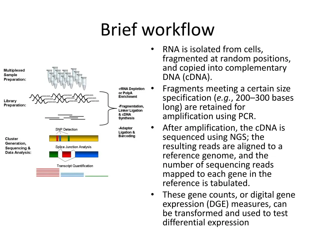
Brief workflow. RNA is isolated from cells, fragmented at random positions, and copied into complementary DNA (cDNA). Fragments meeting a certain size specification ( e.g. , 200–300 bases long) are retained for amplification using PCR.

E N D
Brief workflow • RNA is isolated from cells, fragmented at random positions, and copied into complementary DNA (cDNA). • Fragments meeting a certain size specification (e.g., 200–300 bases long) are retained for amplification using PCR. • After amplification, the cDNA is sequenced using NGS; the resulting reads are aligned to a reference genome, and the number of sequencing reads mapped to each gene in the reference is tabulated. • These gene counts, or digital gene expression (DGE) measures, can be transformed and used to test differential expression
But… many steps in experimental process may introduce errors and biases
FASTQ format • The first line starts with '@', followed by the label • The third line starts with '+'. In some variants, the '+' line contains a second copy of the label • The fourth line contains the Q scores represented as ASCII characters
Scales of genome size Russell F. Doolittle Nature 419, 493-494(3 October 2002)
Exploratory analyses 1.PCA
Exploratory analyses 2.Unsupervised clustering
Exploratory analyses 2b.Unsupervised clustering on gene subset GF Zhang et al. Nature000, 1-6 (2012) doi:10.1038/nature11413
From microarrays to NGS data • As research transitions from microarrays to sequencing-based approaches, it is essential that we revisit many of the same concerns that the statistical community had at the beginning of the microarray era • series of articles was published elucidating the need for proper experimental design
Experimental design • All of these articles rely on the three fundamental aspects of sound experimental design formalized by R. A. Fisher 70 years (!!!) ago, namely replication, randomization, and blocking: the experimental design would include many different subjects (i.e., replication) recruited from multiple weight loss centers (i.e., blocking). Each center would randomly assign its subjects to one of the two diets (i.e., randomization).
In case of bad experimental design • it is essentially impossible to partition biological variation from technical variation • No amount of statistical sophistication can separate confounded factors after data have been collected.
Good news for NGS • certain properties of the platforms can be leveraged to ensure proper design • Capacity to bar code
Replication1. no biological replication • Unreplicated data consider only a single subject per treatment group • it is not possible to estimate variability within treatment group, and the analysis must proceed without any information regarding within-group biological variation Auer P L , and Doerge R W Genetics 2010;185:405-416
Fisher'sexact test • The cell counts represent the DGE count for gene A or the remaining genes, for Treatment 1, and 2. • Several methods for p-value computation
Log2 FC Gene expression counts were normalized by the column totals of the corresponding 2 × 2 table. Blue dots represent significantly differentially expressed genes (by Fisher's exact test); gray dots represent genes with similar expression. Auer P L , and Doerge R W Genetics 2010;185:405-416
Limitations of unreplicated data • complete lack of knowledge about biological variation • without an estimate of variability (i.e., within treatment group), there is no basis for inference (between treatment groups) • the results of the analysis only apply to the specific subjects included in the study
Replication2. replicated data • A multiple flow-cell design based on three biological replicates within seven treatment groups. There are three flow cells with eight lanes per flow cell. The control sample is in lane 5 of each flow cell. Tij refers to the j-th replicate in the i-th treatment group . Auer P L , and Doerge R W Genetics 2010;185:405-416
DGE • methods for testing differential expression that incorporates within-group (or within-treatment) variability relies on a generalized linear model (Poisson GLM, logistic regression models, Bayessian approach, beta binomial model, negative binomial model)
Blocking • if the treatment effects are not separable from possible confounding factors, then for any given gene, there is no way of knowing whether the observed difference in abundance between treatment groups is due to the biology or the technology (e.g., amplification or sequencing bias).
Comparison of two designs Auer P L , and Doerge R W Genetics 2010;185:405-416
0. Cofounded design • typical RNA-Seq experiment • consists of the same six samples, with no bar coding, and does not permit partitioning of batch and lane effects from the estimate of within-group biological variability.
1. Balanced block design • Bar coding results in six technical replicates of each sample, while balancing batch and lane effects and blocking on lane. • Allows partitioning of batch and lane effects from the within-group biological variability.
2. Balanced incomplete block designs and blocking without multiplexing • Mostly reliable • in reality: the number of treatments (I), the number of biol. replicates per treatment (J), the number of unique bar codes (s) that can be included in a single lane, the number of lanes available for sequencing (L).
A balanced incomplete block design (BIBD) for three treatment groups (T1, T2, T3) with one subject per treatment group (T11,T21, T31) and two technical replicates of each (T111, T112,T211, T212,T311, T312). • each of the three samples is bar coded and divided in two (e.g., T11 would be split into T111 and T112) and then pooled and sequenced as illustrated (e.g., T111 is pooled with T212 as input to lane 1). Auer P L , and Doerge R W Genetics 2010;185:405-416
A design based on three biological replicates within seven treatment groups. For each of the three flow cells there are eight lanes per flow cell and a control sample in lane 5. Tij refers to the j-th replicate in the i-th treatment group Auer P L , and Doerge R W Genetics 2010;185:405-416
Overview http://www.nature.com/nprot/journal/v8/n9/full/nprot.2013.099.html
Expression level in RNA-seq = The number of reads (counts) mapping to the biological feature of interest (gene, transcript, exon, etc.) is considered to be linearly related to the abundance of the target feature
What is differential expression? • A gene is declared differentially expressed if an observed difference or change in read counts between two experimental conditions is statistically significant, i.e. whether it is greater than what would be expected just due to natural random variation. • Statistical tools are needed to make such a decision by studying counts probability distributions.
Definitions • Sequencing depth: Total number of reads mapped to the genome. Library size. • Gene length: Number of bases. • Gene counts: Number of reads mapping to that gene (expression measurement)
Experimental design • Pairwise comparisons: Only two experimental conditions or groups are compared. • Multiple comparisons: More than 2 conditions or groups. Replicates • Biological replicates. To draw general conclusions: from samples to population. • Technical replicates. Conclusions are only valid for compared samples.
RNA-seq biases • Influence of sequencing depth: The higher sequencing depth, the higher counts
RNA-seq biases • Dependence on gene length: Counts are proportional to the transcript length times the mRNA expression level %DE genes Oshlack and Wakefield. 2009
RNA-seq biases • Differences on the counts distribution among samples
RNA-seq biases • Influence of sequencing depth: The higher sequencing depth, the higher counts. • Dependence on gene length: Counts are proportional to the transcript length times the mRNA expression level. • Differences on the counts distribution among samples.
Options 1. Normalization: Counts should be previously corrected in order to minimize these biases. 2. Statistical model should take them into account.
Normalization methods • RPKM (Mortazavi et al., 2008) = Reads per kilo base per million: Counts are divided by the transcript length (kb) times the total number of millions of mapped reads • Upper-quartile(Bullard et al., 2010): Counts are divided by upper-quartile of counts for transcripts with at least one read. • TMM (Robinson and Oshlack, 2010): Trimmed Mean of M values. • Quantiles, as in microarray normalization (Irizarry et al., 2003). • FPKM (Trapnell et al., 2010): Instead of counts, Cufflinks software generates FPKM values (Fragments Per Kilobaseof exon per Millionfragmentsmapped) to estimate gene expression, which are analogous to RPKM.
Differential expression • Parametric assumptions: Are they fulfilled? • Needofreplicates. • Problems to detect differential expression in genes with low counts.
Goal • Based on a count table, we want to detect differentially expressed genes between conditions ofinterest. • We will assign to each gene a p-value (0-1), which shows us 'how surprised we should be' to see this difference, when we assume there is no difference.
Algorithms under active development http://wiki.bits.vib.be/index.php/RNAseq_toolbox#Detecting_differential_expression_by_count_analysis
Intuition - gene } Variability A Variability B CompareandconcludegivenaMeanlevel:similarornot?
Intuition NB model is estimated: 2 parameters needed (mean and dispersion)
Intuition Difference is quantified and used for p-value computation
Dispersion estimation • For every gene, a NB is fitted based on the counts. The most important factor in that model to be estimated is the dispersion. • DESeq2 estimates dispersion by 3 steps: 1. Estimates dispersion parameter for each gene 2. Plots and fits a curve 3. Adjusts the dispersion parameter towards the curve ('shrinking')
Dispersion estimation • Black dots = estimates from the data • Red line = curve fitted • Blue dots = final assigned dispersion parameter for that gene Model is fitted
Test runs between 2 conditions • for each gene 2 NB models (one for each condition) are made, and a Wald test decides whether the difference is significant (red in plot).
Test runs between 2 conditions • for each gene 2 NB models (one for each condition) are made, and a Wald test decides whether the difference is significant (red in plot). i.e. we are going to perform thousands of tests… (if we set set a cut-off on the p-value of 0,05 and we have performed 20000 tests, 1000 genes will appear significant by chance)
Check the distribution of p-values • If the histogram of the p-values does not match a profile as shown here, the test is not reliable. Perhaps the NB fitting step did not succeed, or confounding variables are present.