Download
1 / 24
240 likes | 331 Views
Clustering. “ Are there clusters of similar cells?”. Light color with 1 nucleus. Dark color with 2 tails 2 nuclei. 1 nucleus and 1 tail. Dark color with 1 tail and 2 nuclei. Association Rule Discovery. Task: Discovering association rules among items in a transaction database.

E N D
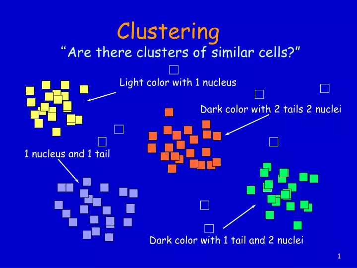
Clustering “Are there clusters of similar cells?” Light color with 1 nucleus Dark color with 2 tails 2 nuclei 1 nucleus and 1 tail Dark color with 1 tail and 2 nuclei
Association Rule Discovery Task: Discovering association rules among items in a transaction database. An association among two items A and B means that the presence of A in a record implies the presence of B in the same record: A => B. In general: A1, A2, … => B
Association Rule Discovery “Are there any associations between the characteristics of the cells?” If color = light and # nuclei = 1 then # tails = 1(support = 12.5%; confidence = 50%) If # nuclei = 2 and Cell = Cancerous then # tails = 2 (support = 25%; confidence = 100%) If # tails = 1 then Color = light(support = 37.5%; confidence = 75%)
Many Other Data Mining Techniques Genetic Algorithms Statistics Bayesian Networks Text Mining Time Series Rough Sets
Lecture 1: Overview of KDD 1. What is KDD and Why ? 2. The KDD Process 3. KDD Applications 4. Data Mining Methods 5. Challenges for KDD
Challenges and Influential Aspects Handling of different types of data with different degree of supervision Massive data sets, high dimensionality (efficiency, scalability) Different sources of data (distributed, heterogeneous databases, noise and missing, irrelevant data, etc.) Interactive, Visualization Knowledge Discovery Understandability of patterns, various kinds of requests and results (decision lists, inference networks, concept hierarchies, etc.) Changing data and knowledge
Massive Data Sets and High Dimensionality # attributes ? Cancerous Cell • High dimensionality increases exponentially the size of the space of patterns. C2 C1 C3 Healthy Cell h2 h1 With p attributes each has d discrete values in average, the space of possible instances has the size of dp. Classes: {Cancerous, Healthy} Attributes: Cell body: {dark, light} #nuclei: {1, 2} #tails: {1, 2} 38 attributes, each 10 values # instances = 1038 (# instances = 23 = 8)
Different Types of Data Combinatoricalsearch in hypothesis spaces (machine learning) Attribute Numerical Symbolic No structure Nominal (categorical) Ordinal Measurable Places, Color Ordinal structure Age, Temperature, Taste, Rank, Resemblance Ring structure Income, Length Often matrix-based computation (multivariate data analysis)
Brief introduction to lectures Lecture 1: Overview of KDD Lecture 2: Preparing data Lecture 3: Decision tree induction Lecture 4: Mining association rules Lecture 5: Automatic cluster detection Lecture 6: Artificial neural networks Lecture 7: Evaluation of discovered knowledge
Lecture 2: Preparing Data • As much as 80% of KDD is about preparing data, and the remaining 20% is about mining • Content of the lecture 1. Data cleaning 2. Data transformations 3. Data reduction 4. Software and case-studies • Prerequisite: Nothing special but expected some understanding of statistics
Data Preparation The design and organization of data, including the setting of goals and the composition of features, is done by humans. There are two central goals for the preparation of data: • To organize data into a standard form that is • ready for processing by data mining programs. • To prepare features that lead to the best • data mining performance.
Brief introduction to lectures Lecture 1: Overview of KDD Lecture 2: Preparing data Lecture 3: Decision tree induction Lecture 4: Mining association rules Lecture 5: Automatic cluster detection Lecture 6: Artificial neural networks Lecture 7: Evaluation of discovered knowledge
Lecture 3: Decision Tree Induction • One of the most widely used KDD classification techniques for supervised data. • Content of the lecture • 1. Decision tree representation and framework • 2. Attribute selection • 3. Pruning trees • 4. Software C4.5, CABRO and case-studies • Prerequisite: Nothing special
Decision Trees Decision Tree is a classifier in the form of a tree structure that is either: • a leaf node, indicating a class of instances, or • a decision node that specifies some test to be carried out on a single attribute value, with one branch and subtree for each possible outcome of the test A decision tree can be used to classify an instance by starting at the root of the tree and moving through it until a leaf is met.
General Framework of Decision Tree Induction 1. Choose the “best” attribute by a given selection measure 2. Extend tree by adding new branch for each attribute value 3. Sorting training examples to leaf nodes 4. If examples unambiguously classified Then Stop Else Repeat steps 1-4 for leaf nodes 5. Pruning unstable leaf nodes Temperature Flu Temperature Headache normal veryhigh high {e1, e4} e1 yes normal no {e2, e5} {e3,e6} e2 yes high yes no Headache Headache e3 yes very high yes e4 no normal no yes {e2} yes {e3} no {e6} no {e5} e5 no high no yes no e6 no very high no yes no
Avoiding Overfitting How can we avoid overfitting? • Stop growing when data split not statistically • significant (pre-pruning) • Grow full tree, then post-prune (post-pruning) Two post-pruning techniques • Reduce-Error Pruning • Rule Post-Pruning
Converting A Tree to Rules outlook sunny o’cast rain wind yes humidity true false high normal no yes no yes IF (Outlook = Sunny) and (Humidity = High) THEN PlayTennis = No IF (Outlook = Sunny) and (Humidity = Normal) THEN PlayTennis = Yes ........
CABRO: Decision Tree Induction CABRO based on R-measure, a measure for attribute dependency stemmed from rough sets theory. Discovered decision tree Matching path and the class that matches the unknown instance Unknown case
Brief introduction to lectures Lecture 1: Overview of KDD Lecture 2: Preparing data Lecture 3: Decision tree induction Lecture 4: Mining association rules Lecture 5: Automatic cluster detection Lecture 6: Artificial neural networks Lecture 7: Evaluation of discovered knowledge
Lecture 4: Mining Association Rules • A new technique and attractive topic. It allows discovering the important associations among items of transactions in a database. • Content of the lecture • Prerequisite: Nothing special 1. Basic Definitions 2. Algorithm Apriori 3. The Basket Analysis Program
Measures of Association Rules There are two measures of rule strength: Support of (A => B) = [AB] / N, where N is the number of records in the database. The support of a rule is the proportion of times the rule applies. Confidence of (A => B) = [AB] / [A] The confidence of a rule is the proportion of times the rule is correct.
Algorithm Apriori • The task of mining association rules is mainly to discover strong association rules (high confidence and strong support) in large databases. TID Items 1000 A, B, C 2000 A, C 3000 A, D 4000 B, E, F • Mining association rules is composed • of two steps: • 1. discover the large items, i.e., the • sets of itemsets that have • transaction support above a • predetermined minimum support s. • 2. Use the large itemsets to generate • the association rules Large support items {A} 75% {B} 50% {C} 50% {A,C} 50% S = 40%
Algorithm Apriori: Illustration C1 L1 Database D S = 40% Itemset Count {A} {B} {C} {D} {E} Itemset Count {A} 2 {B} 3 {C} 3 {E} 3 TID Items 100 A, C, D 200 B, C, E 300 A, B, C, E 400 B, E 2 Scan D 3 3 1 3 C2 C2 L2 {A, B} {A, C} {A, E} {B, C} {B, E} {C, E} Itemset {A, B} {A, C} {A, E} {B, C} {B, E} {C, E} Itemset Count {A, C} 2 {B, C} 2 {B, E} 3 {C, E} 2 Itemset Count 1 Scan D 2 1 2 3 2 C3 C3 L3 Scan D {B, C, E} Itemset {B, C, E} 2 {B, C, E} 2 Itemset Count Itemset Count


![[virtual] cells](https://cdn1.slideserve.com/3553683/slide1-dt.jpg)