Download
1 / 72
720 likes | 849 Views
Томск 16-25.07.2004. Современные вычислительные технологии в задачах прогноза погоды. Г.С.Ривин. Rivin@ict.nsc.ru. www.ict.nsc.ru. ATMOSPHERIC PROCESSES in SPACE-ATMOSPHERE-SEA/LAND system. Submodels. WMO WEATHER FORECASTING RANGES. COMPONENTS of FORECAST SYSTEM.

E N D
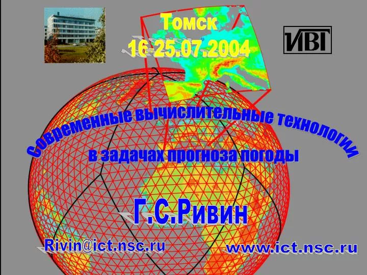
Томск 16-25.07.2004 Современные вычислительные технологии в задачах прогноза погоды Г.С.Ривин Rivin@ict.nsc.ru www.ict.nsc.ru
COMPONENTS of FORECAST SYSTEM 1. Observing system 2. Telecommunication system 3. Computer system 4. Data assimilation 5. Model 6. Postprocessing
Observing System SYNOP AIROCRAFS AIROLOGICAL DATA
Observing System RADARS, r = 100km Radar
The system of equations(conservation laws applied to individual parcels of air) (from E.Kalnay) • conservation of the 3-dimensional momentum (equations of motion), • conservation of dry air mass (continuity equation), • the equation of state for perfect gases, • conservation of energy (first law of thermodynamics), • equations for the conservation of moisture in all its phases. They include in their solution fast gravity and sound waves, and therefore in their space and time discretization they require the use of smaller time steps, or alternative techniques that slow them down. For models with a horizontal grid size larger than 10 km, it is customary to replace the vertical component of the equation of motion with its hydrostatic approximation, in which the vertical acceleration is neglected compared with gravitational acceleration (buoyancy). With this approximation, it is convenient to use atmospheric pressure, instead of height, as a vertical coordinate. V. Bjerknes (1904) pointed out for the first time that there is a complete set of 7 equations with 7 unknowns that governs the evolution of the atmosphere:
2003, December MODELS of ATMOSPHERE ECMWF: T511L60 – 40 km; EPS: T255L60 – 80 km; DWD: GME (L41) – 40 km; LM (L3550) – (2.8)7 km; France: ARPEGE(L41)-23-133km; ALADIN (L41)– 9 km; HIRLAM: -------------- (L16-31) – 5-55 km; UK: UM(L30) – 60 km; (L38) – 12 km; USA: AVP (T254L64) – 60 km; ETA (L60) – 12 km; Japan: GSM(L40) – 60 km; MSM(L40) – 10 km. RusFed.: T85L31 – 150 km; (L31) – 75 km. Moscow region (300kmx300km) - 10 km.
Coordinate systems: p, sigma, z, eta, hybrid Models of atmosphere: Steps: global - 40-60 km, local 7-12 km; Methods: splitting, semi-Lagrangian scheme (23), ensembles, nonhydrostatic, grids Data assimilation: 3(4)D-Var, Kalman filter Reanalyses NCEP / NCAR USA50-years (1948-…; T62L28~210km) Reanalyses-2 (ETA RR 32 km, 45 layers)ECMWF ERA-15 (TL106L31~150km, 1979-1993), ERA-40 (TL159L60~120km, 3D-Var, mid1957-2001) FEATURES OF INFORMATION AND COMPUTATIONAL TECHNOLOGIES IN ATMOSPHERIC SCIENCES
Modern and Possible further development computational technologies ensemble simulation
ECMWF: FORECASTING SYSTEM - DECEMBER 2003 Model: Smallest half-wavelength resolved: 40 km (triangular spectral truncation 511) Vertical grid: 60 hybrid levels (top pressure: 10 Pa) Time-step: 15 minutes Numerical scheme:Semi-Lagrangian, semi- implicit time-stepping formulation. Number of grid points in model: 20,911,680 upper-air, 1,394,112 in land surface and sub- surface layers. The grid for computation of physical processes is a reduced, linear Gaussian grid, on which single- level parameters are available. The grid spacing is close to 40km. Variables at each grid point (recalculated at each time-step): Wind, temperature, humidity, cloud fraction and water/ ice content, ozone content (also pressure at surface grid-points) Physics: orography (terrain height and sub-grid-scale), drainage, precipitation, temperature, ground humidity, snow-fall, snow-cover & snow melt, radiation (incoming short-wave and out-going long-wave), friction (at surface and in free atmosphere), sub-grid-scale orographic drag - gravity waves and blocking effects, evaporation, sensible & latent heat flux, oceanic waves.
ECMWF: FORECASTING SYSTEM - DECEMBER 2003 Data Assimilation: Analysis: Mass & wind (four-dimensional variational multi- variate analysis on 60 model levels) Humidity (four-dimensional variational analysis on model levels up to 250 hPa) Surface parameters (sea surface temperature from NCEP Washington analysis, sea ice from SSM/I satellite data), soil water content, snow depth, and screen level temperature and humidity Data used: Global satellite data (SATOB/AMV, (A)TOVS, Quikscat, SSM/I, SBUV, GOME, Meteosat7 WV radiance), Global free-atmosphere data (AIREP, AMDAR, TEMP, PILOT, TEMP/DROP, PROFILERS), Oceanic data (SYNOP/SHIP, PILOT/SHIP, TEMP/SHIP, DRIBU), Land data (SYNOP). Data checking and validation is applied to each parameter used. Thinning procedures are applied when observations are redundant at the model scale.
Nonhydrostatic models • the Penn State/NCAR Mesoscale Model (e.g., Dudhia, 1993), • the CAPS Advanced Regional prediction System (Xue et al, 1995), • NCEP's Regional Spectral Model (Juang et al, 1997), • the Mesoscale Compressible Community (MCC) model (Laprise et al, 1997), • the CSU RAMS Tripoli and Cotton (1980), • the US Navy COAMPS (Hodur, 1997).
WRF Development Teams WG8 WG1 WG3 WG6 WG12 WG5 WG9 WG4 WG7 WG2 WG11 WG15 WG14 WG10 WG13 WG16 Courtesy NCAR
1 10 100 km Resolved Convection Cumulus Parameterization 3-D Radiation Two Stream Radiation LES PBL Parameterization Model Physics in High Resolution NWP Physics “No Man’s Land” From Joe Klemp, NCAR (Bad Orb, 23-27.10.03 2003)
36h WRF Precip Forecast Analyzed Precip 27 Sept. 2002 Weather Research and Forecasting Model Goals: Develop an advanced mesoscale forecast and assimilation system, and accelerate research advances into operations • Collaborative partnership, principally amongNCAR, NOAA, • DoD, OU/CAPS, FAA, and university community • Multi-agency WRF governance; development conducted • by 15 WRF Working Groups • Software framework provides portable, scalable code with • plug-compatible modules • Ongoing active testing and rapidly growing community use • Over 1,400 registered community users, annual • workshops and tutorials for research community • Daily experimental real-time forecasting at NCAR , • NCEP, NSSL, FSL, AFWA, U. of Illinois • Operational implementation at NCEP and AFWA in FY04 From Joe Klemp, NCAR (Bad Orb, 23-27.10.03 2003)
Hurricane Isabel NOAA –17 AVHRR 13 Sep 03 14:48 GMT From Joe Klemp, NCAR (Bad Orb, 23-27.10.03 2003)
Hurricane Isabel Track 18/1700Z 4 km WRF Initialized 17/0000Z 10 km WRF Initialized 15/1200Z From Joe Klemp, NCAR (Bad Orb, 23-27.10.03 2003)
Hurricane Isabel 3 h Precip Forecast WRF Model 10 km grid 5 day forecast Initialized: 12 UTC 15 Sep 03 From Joe Klemp, NCAR (Bad Orb, 23-27.10.03 2003)
48 h Hurricane Isabel Reflectivity Forecast Initialized 00 UTC 17 Sep 03 Radar Composite 4 km WRF forecast From Joe Klemp, NCAR (Bad Orb, 23-27.10.03 2003)
Hurricane Isabel Reflectivity at Landfall 18 Sep 2003 1700 Z 41 h forecast from 4 km WRF Radar Composite From Joe Klemp, NCAR (Bad Orb, 23-27.10.03 2003)
Hurricane Isabel Surface-Wind Forecast WRF Model 4 km grid 2 day forecast Initialized: 00 UTC 17 Sep 03 From Joe Klemp, NCAR (Bad Orb, 23-27.10.03 2003)
WRF Mass Coordinate Core • Terrain-following hydrostatic pressure vertical coordinate • Arakawa C-grid, two-way interacting nested grids (soon) • 3rd order Runge-Kutta split-explicit time differencing • Conserves mass, momentum, dry entropy, and scalars • using flux form prognostic equations • 5th order upwind or 6th order centered differencing • for advection • Physics for CR applications: Lin microphysics, YSU PBL, • OSU/MM5 LSM, Dudhia shortwave/RRTM longwave • radiation, no cumulus parameterization From Joe Klemp, NCAR (Bad Orb, 23-27.10.03 2003)
Model Configuration for 4 km Grid • Domain • 2000 x 2000 km, 501 x 501 grid • 50 mb top, 35 levels • 24 s time step • Initialization • Interpolated from gridded analyses • BAMEX: 40 km Eta CONUS analysis • Isabel: 1o GFS global analysis (~110 km) • Computing requirements • 128 Processors on IBM SP Power 4 Regatta • Run time: 106 min/24h of forecast From Joe Klemp, NCAR (Bad Orb, 23-27.10.03 2003)
Prediction Model Data Assimilation Date 12 km Meso Eta 12 km 3DVAR radial velocity 9/30/2002 10 km Meso Eta improved physics 10 km hourly update & improved background error cov. 2/28/2004 9 km NMM top @ 2mb hourly output 9 km AIRS, GOES imagery & move top to 2mb 5/31/2005 8 km WRF 8 km WRF 4DDA 5/31/2006 7 km WRF improved physics 7 km absorption scattering in radiative transfer 5/31/2008 6 km WRF aerosols 6 km aerosols in radiative transfer & reflectivity 5/31/2009 5 km WRF L100 5 km NPP, advanced 4DDA, NPOESS, IASI & air quality 5/31/2010 North American Early Guidance System
Prediction Model Data Assimilation Date T-254 / L64 3D-VAR, AMSU-B, Quikscat 9/30/2002 T-254 / L64 add 2 passive tracers Grid point version, AIRS, GOES imagery 2/28/2004 45 km / L64 3-D Background error covariance, cloud analysis, minimization 5/31/2005 45 km / L64 + improved microphysics Absorption / scattering in radiative transfer 5/31/2006 40 km / L80 Aerosols in radiative transfer, GIFTS 5/31/2008 40 km / L80 NPP, integrated SST analysis 5/31/2009 35 km / L100 Advanced 4DDA, NPOESS, IASI + air quality 5/31/2010 Global Forecast System (GFS)
Timeline for WRF at NCEP • North American WRF: Operational in FY05 • Hurricane WRF: Operational in FY06 • Rapid Refresh (RUC) WRF (hourly): Operational in FY07 • WRF SREF : Operational in FY07 • Others? (Fire Wx, Homeland Security,etc.) using best WRF deterministic model
http://www.metoffice.com/research/nwp/numerical/unified_model/index.htmlhttp://www.metoffice.com/research/nwp/numerical/unified_model/index.html The Unified Model The Unified Model is the name given to the suite of atmospheric and oceanic numerical modelling software developed and used at the Met Office. The formulation of the model supports global and regional domains and is applicable to a wide range of temporal and spatial scales that allow it to be used for both numerical weather prediction and climate modelling as well as a variety of related research activities. The Unified Model was introduced into operational service in 1992. Since then, both its formulation and capabilities have been substantially enhanced. New DynamicsA major upgrade to the Met Office Global Numerical Weather Prediction model was implemented on 7th August 2002. SubmodelsThe Unified Model is made up of a number of numerical submodels representing different aspects of the earth's environment that influence the weather and climate. Like all coupled models the Unified Model can be split up in a number of different ways, with various submodel components switched on or off for a specific modelling application. The Portable Unified Model (PUM)A portable version of the Unified Model has also been developed suitable for running on workstations and other computer systems.
http://www.metoffice.com/research/nwp/numerical/unified_model/new_dynamics.htmlhttp://www.metoffice.com/research/nwp/numerical/unified_model/new_dynamics.html • The Met Office Global Numerical Weather Prediction model • was implemented on 7th August 2002. • The package of changes was under trial for over a year and is known as "New Dynamics". • This document details some of the key changes that are part of the New Dynamics package. • Non-hydrostatic model with height as the vertical co-ordinate. • Charney-Philips grid-staggering in the vertical, • Arakawa C-grid staggering in the horizontal, • Two time-level, semi-Lagrangian advection and semi-implicit time stepping. • Edwards-Slingo radiation scheme with non-spherical ice spectral files • Large-scale precipitation includes prognostic ice microphysics. • Vertical gradient area large-scale cloud scheme. • Convection with convective available potential energy (CAPE) closure, momentum transports and convective anvils. • A boundary-layer scheme which is non-local in unstable regimes. • Gravity-wave drag scheme which includes flow blocking. • GLOBE orography dataset. • The MOSES (Met Office Surface Exchange Scheme) surface hydrology and soil model scheme. • Predictor-corrector technique with no extraction of basic state profile. • Three-dimensional Helmholtz-type equation solved using GCR technique.
Météo-France 2003 status The operational forecast system at Météo-France is based on two different numerical applications of the same code 1. ARPEGE-IFS, 2. additional code to build the limited area model ALADIN. The ARPEGE-IFS has been developed jointly by Météo-France and ECMWF (ARPEGE is the usual name in Toulouse and IFS - in Reading): ECMWF model for medium range forecasts (4-7 days) a Toulousevariable mesh version in for short range predictions (1-4 days) The ALADIN library has been developed jointly by Météo-France and the national meteorological or 14 hydrometeorological services: Austria, Belgium, Bulgaria, Croatia, Czech Republic, Hungary, Moldova, Morocco, Poland, Portugal, Romania, Slovakia, Slovenia, Tunisia.
Local model (LM) 40(35) 325 35 325 Global model (GME) DWD FORECAST SYSTEM
DWD FORECAST SYSTEM Global model (GME)
Local model (LM) DWD FORECAST SYSTEM
Further Development of the Local Systems LME and LMK 2003 to 2006 LME: Local model LM for whole of Europe; mesh size 7 km and 40 layers; 78-h forecasts from 00, 12 and 18 UTC. LMK: LM-”Kürzestfrist”; mesh size < 3 km and 50 layers; 18-h forecasts from 00, 03, 06, 09, 12, 15, 18, 21 UTC for Germany with explicit prediction of deep convection. 1. Data assimilation • 2 Q 2005 • Use satellite (GPS) and radar data (reflectivity, VAD winds) • 1 Q 2006 • Use European wind profiler and satellite data
Further Development of the Local Systems LME and LMK 2003 to 2006 2. Local modelling • 2 Q 2004 • Increase model domain (7 km mesh) from 325x325up to753x641 gridpoints (covering whole of Europe), 40 layers • 3 Q 2005 • New convection scheme (Kain-Fritsch ?)
LMK: LM-Kürzestfrist Model-based system for nowcasting and very short range forecasting Goals: Prediction of severe weather on the mesoscale. Explicit simulation of deep convection. Method: 18-h predictions of LM initialised every three hours, mesh size < 3 km Usage of new observations: SYNOP: Every 60 min, METAR: Every 30 min, GPS: Every 30 min, VAD winds: Every 15 min, Reflectivity: Every 15 min, Wind profiler: Every 10 min, Aircraft data.
+18h +15h +12h +9h +6h +3h 00 03 06 09 12 15 18 21 00 (UTC) LMK: A new 18-h forecast every three hours
High-resolution Regional Model HRM • Operational NWP Model at 13 services worldwide • Hydrostatic, (rotated) latitude/longitude grid • Operators of second order accuracy • 7 to 28 km mesh size, various domain sizes • 20 to 35 layers (hybrid, sigma/pressure) • Prognostic variables: ps, u, v, T, qv, qc, qi • Same physics package as GME • Programming: Fortran90, OpenMP/MPI for parallelization • From 00 and 12 UTC: Forecasts up to 78 hours • Lat. bound. cond. from GME at 3-hourly intervals
General structure of a regional NWP system Topographical data Graphics Visualization MOS Kalman Regional NWP Model Initial data (analysis) Direct model output (DMO) Applications Wave model, Trajectories Lateral boundary data Verification Diagnostics
Prognostic variables Surface pressure ps Temperature T Water vapour qv Cloud water qc Cloud ice qi Horizontal wind u, v Several surface/soil parameters Diagnostic variables Vertical velocity Geopotential Cloud cover clc Diffusion coefficients tkvm/h Short Description of the High-Resolution Regional Model (HRM)Hydrostatic limited-area meso- and meso- scale numerical weather prediction model
Brazil, Directorate of Hydrography & Navigation Brazil, Instituto Nacional de Meteorologia Bulgaria, National Meteoro-logical & Hydrological Service China, Guangzhou Regional Meteorological Centre India, Space Physics Lab. Israel, Israel Meteorological Service Italy, Italian Meteorological Service Kenya, National Meteorological Service Oman, National Meteoro-logical Service (DGCAM) Romania, National Meteoro-logical & Hydrological Service Spain, National Met. Institute United Arab Emirates, National Met. Institute Vietnam, National Meteoro-logical & Hydrological Service; Hanoi University Current operational users of the HRM
Numerics of the HRM • Regular or rotated latitude/longitude grid • Mesh sizes between 0.25° and 0.05° (~ 28 to 6 km) • Arakawa C-grid, second order centered differencing • Hybrid vertical coordinate, 20 to 35 layers • Split semi-implicit time stepping; t = 150s at = 0.25° • Lateral boundary formulation due to Davies • Radiative upper boundary condition as an option • Fourth-order horizontal diffusion, slope correction • Adiabatic implicit nonlinear normal mode initialization