Download
1 / 15
150 likes | 284 Views
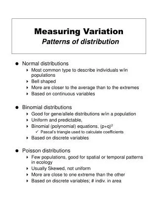
Measuring Variation 2. Lecture 17 Sec. 5.3.3 Mon, Feb 14, 2005. The Five-Number Summary. Five-number summary – A summary of a sample or population consisting of the five numbers Minimum First quartile Q1 Median Third quartile Q3 Maximum

E N D
Measuring Variation 2 Lecture 17 Sec. 5.3.3 Mon, Feb 14, 2005
The Five-Number Summary • Five-number summary – A summary of a sample or population consisting of the five numbers • Minimum • First quartile Q1 • Median • Third quartile Q3 • Maximum • This does a better job of measuring spread than any single number can do.
TI-83 – Five-Number Summary • Use the TI-83 to find a five-number summary of the age data. • Min = 32 • Q1 = 41 • Median = 43.5 • Q3 = 46.5 • Max = 51
The Five-Number Summary • From the 5-number summary of the age data, can we detect skewness in the distribution? • Answer: Maybe.
Boxplots • Boxplot – A graphical display of a five-number summary. • Draw and label a scale representing the variable. • Draw a box over the scale with its left and right ends at Q1 and Q3. • Draw a vertical line through the box at the median. • Draw a left tail (whisker) from the box to the minimum. • Draw a right tail from the box to the maximum.
Example • Draw a boxplot of the age data.
Boxplots and Shape • What would a boxplot for a uniform distribution look like? • What would a boxplot for a symmetric distribution look like? • What would a boxplot for a left-skewed distribution look like?
TI-83 – Boxplots • Press STAT PLOT. • Select Plot1 • Turn Plot 1 On. • Select the Boxplot Type. • Specify list L1. • Press WINDOW. • Set minX and maxX appropriately. • Press GRAPH. • See the instructions on p. 283.
TI-83 – Boxplots • Press TRACE. • Use the arrow keys to see the values of the minimum, Q1, the median, Q3, and the maximum.
Modified Boxplots • Modified boxplot – A boxplot in which the outliers are indicated.
Modified Boxplots • Draw the box part of the boxplot as usual. • Compute STEP = 1.5 IQR. • The inner fences are at Q1 – STEP and Q3 + STEP. • Extend the whiskers from the box to the smallest and largest values that are within the inner fences. • Draw as individual dots any values that are outside the inner fences. These dots represent outliers.
Example: DePaul University • For an example of modified boxplots, see DePaul University’s web page on retention.
Example • Draw a modified boxplot of the age data. • Do the age data have any outliers? • See Example 5.6, p. 286.
TI-83 – Modified Boxplots • Follow the same steps as for a regular boxplot, but for the Type, select the modified-boxplot icon, the first icon in the second row. • It looks like a boxplot with a couple of extra dots. • Use the TI-83 to find a modified boxplot of the age data.
Let’s Do It! • Let’s do it! 5.9, p. 286 – Five-number Summary and Outliers. • Let’s do it! 5.10, p. 287 – Cost of Running Shoes. • Let’s do it! 5.11, p. 288 – Comparing Ages– Antibiotic Study.