Download
1 / 9
130 likes | 506 Views
Lazy learning vs. eager learning. Processing is delayed until a new instance must be classified Pros: Classification hypothesis is developed locally for each instance to be classified Cons: Running time (no model is built, so each classification actually builds a local model from scratch).

E N D
Lazy learning vs. eager learning • Processing is delayed until a new instance must be classified • Pros: • Classification hypothesis is developed locally for each instance to be classified • Cons: • Running time (no model is built, so each classification actually builds a local model from scratch)
K-Nearest Neighbors • Classification of new instances is based on classifications of (one or more) known instances nearest to them • K=1 1-NN (using a single nearest neighbor) • Frequently, K > 1 • Assumption: all instances correspond to points in the n-dimensional space Rn • Dimensions = features (aka attributes)
Metrics • Nearest neighbors are identified using a metric defined for this high-dimensional space • Let x be an arbitrary instance with feature vector <f1(x), f2(x), …, fn(x)> • Euclidean metric is frequently used for real-valued features:
Pseudo-code for KNN • Training algorithm • For each training example <x, class(x)>, add the example to the list Training • Classification algorithm (Rn V) • Let V ={v1, …, vl} be a set of classes • Given a query instance xq to be classified • Let X={x1, …, xk} denote the k instances from Training that are nearest to xq • Return vi such that |votei|is largest
Distance-weighted KNN • Weighting contribution of each of the k neighbors according to their distance to the query point xq • Give greater weight to closer neighbors • Return vi such that |wi|is largest
Distance-weighted KNN (cont’d) • If xq exactly matches one of the training instances xi, and d(xq, xi)=0, • then we simply take class(xi) to be the classification of xq
Remarks on KNN • Highly effective learning algorithm • The distance between instances is calculated based on all features • If some features are irrelevant, or redundant, or noisy, then KNN suffers from the curse of dimensionality • In such a case, feature selection must be performed prior to invoking KNN
Home assignment #4: Feature selection • Compare the following algorithms • ID3 – regular ID3 with internal feature selection • KNN.all – KNN that uses all the features available • KNN.FS – KNN with a priori feature selection (IG) • Two datasets: • Spam email • Handwritten digits • You don’t have to understand the physical meaning of all the coefficients involved !
Cross-validation • Averaging the accuracy of a learning algorithm over a number of experiments • N-fold cross-validation: • Partition the available data D into N disjoint subsets T1, …, TN of equal size (|D| / N) • For n from 1 to N do • Training = D \ Ti , Testing = Ti • Induce a classifier using Training, test it on Testing, and measure the accuracy Ai • Return (∑ Ai ) / N (cross-validated accuracy)