Download
1 / 15
150 likes | 248 Views
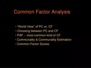
Common Factor Analysis. “World View” of PC vs. CF Choosing between PC and CF PAF -- most common kind of CF Communality & Communality Estimation Common Factor Scores. World View of PC Analyses. PC analysis is based on a very simple “world view” We measure variables

E N D
Common Factor Analysis “World View” of PC vs. CF Choosing between PC and CF PAF -- most common kind of CF Communality & Communality Estimation Common Factor Scores
World View of PC Analyses PC analysis is based on a very simple “world view” • We measure variables • The goal of factoring is data reduction • determine the # of kinds of information in the variables • build a PC for each • R holds the relationships between the variables • PCs are composite variables computed from linear combinations of the measured variables
World View of CF Analyses CF is based on a somewhat more complicated and “causal” world view • Any domain (e.g., intelligence, personality) has some set of “latent constructs” • A person’s “values” on these “latent constructs” causes their scores on any measured variable(s) • any variable has two parts • “common part” -- caused by values of the latent constructs” • “unique part” -- not related to any latent construct (“error”)
World View of CF Analyses, cont • the goal of factoring is to reveal the number and identify of these “latent constructs” • R must be “adjusted” to represent the relationships between portions of the variables that are produced by the “latent constructs” • represent the correlations between the “common” parts of the variables • CFs are linear combinations of the “common” parts of the measured variables that capture the underlying constructs”
Example of CF world view “latent constructs” IQ Math Ability Reading Skill Social Skills “measures” adding, subtraction, multiplication vocabulary, reading speed, reading comprehension politeness, listening skills, sharing skills Each measure is “produced” by a weighted combination of the latent constructs, plus something unique to that measure . . . adding = .5*IQ +.8*Math + 0*Reading + 0*Social + Ua subtraction = .5*IQ +.8*Math + 0*Reading + 0*Social + Us vocabulary = .5*IQ + 0*Math + .8*Reading + 0*Social + Uv politeness = .4*IQ + 0*Math + 0*Reading +.8*Social + Up
Example of CF world view, cont When we factor these, we might find something like CF1 CF2 CF3 CF4 adding .4 .6 subtraction .4 .6 multiplication .4 .6 vocabulary .4 .6 reading speed .4 .6 reading comp .4 .6 politeness .3 .6 listening skills .3 .6 sharing skills .3 .6 Name each “latent construct” that was revealed by this analysis
Principal Axis Analysis “Principal” again refers to the extraction process • each successive factor is orthogonal and accounts for the maximum available covariance among the variables “Axis” tells us that the factors are extracted from a “reduced” correlation matrix • diagonals < 1.00 • diagonals = the estimated “communality” of each variable • reflecting that not all of the variance of that variable is “produced” by the set of “latent variables” • So, factors extracted from the “reduced” R will reveal the latent variables
Which model to choose -- PC or PAF ? Traditionally... PC is used for “psychometric” purposes • reduction of collinear predictor sets • examination of the structure of “scoring systems” • consideration of scales and sub-scales • works with full R because composites will be computed from original variable scores not “common parts” CF is used for “theoretical” purposes • identification of “underlying constructs” • number and identity of “basic elements of behavior” • The basis for “latent class” analyses of many kinds • both measurement & structural models • works with reduced R because it hold the “meaningful” part of the variables and their interrelationships The researcher selects the procedure based on their purpose for the factor analysis !!
Communality & Its Estimation The communality of a variable is the proportion of that variable’s variance that is produced by the common factors underlying the set of variables Common Estimations • (reliability coefficient) -- only the reliable part of the variable can be common • largest r (or r2) with another in the set -- at least that much is shared with other variables • R2 predicting that variable from all the others -- tells how much is shared with other variables Note how the definition shifts from “variance shared with the latent constructs” to “variance shared with the other variables in the set” !! • )\
Communality & Its Estimation: How SPSS does it… Step 1: Perform a PC analysis • extract # PCs from the full R matrix Step 2: Perform 1st PAF Iteration • Use R2 predicting each variable from others -- put in diagonal of R • extract same # PAFs from that reduced R matrix • compute (output) variable communalities Step 3: Perform 2nd PAF Iteration • use variable (output) communalities from last PAF step as estimated (input) communalities -- put in diagonals of R • extract same # PAFs from that reduced R matrix • compute (output) variable communalities • Compare estimated (input) and computed (output) variable communalities Additional Steps: Iterate to convergence of estimated (input) & computed (output) variable communalities
Communality & Its Estimation How SPSS does it…, cont Huh?!!? The idea is pretty simple (and elegant) … • If the communality estimates are correct, then they will be returned from the factor analysis ! • So, start with a “best guess” of the communalities, and iterate until the estimates are stable Note: This takes advantages of the “self-correcting” nature of this iterative process • the initial estimates have very little effect on the final communalities (R2 really easy to calculate) • starting with the PC communalities tends to work quickly Note: This process assumes the latent constructs are adequately represented by the variable set !!
Problems estimating communalities in a CF analysis “failure to converge” • usually this can be solved by increasing the number of iterations allowed (=1000) “Heywood case” λ > 1.00 • During iteration communality estimates can become larger than 1.00 • However no more than “all” of a variable’s variance can be common variance! • Usual solutions… • Use the solution from the previous iteration • Drop the offending variable • If other variables are “threatening to Heywood” consider aggregating them together into a single variable
Common Factor Scores • The “problem” is that common factors can only be computed as combinations of the “common parts” of the variables • Unfortunately, we can’t separate each person’s score on each variable into the “common” and “unique” part • So, common factor scores have to be “estimated” • Good news -- • the procedure used by SPSS works well and is well accepted • since CF is done for “theory testing” or to “reveal latent constructs” rather than for “psychometric purposes” scores for CFs are not used as often as are PC scores
Maximum Likelihood method of Common Factoring • Both PAF & ML are “common factor” extractions • they both seek to separate the “common” vs. “unique” portion of each variable’s variance and include only the common in R • they both require communality estimates • they both iterate communality input estimates & output computations until these two converge, though the process for computing estimates is somewhat different • which is taken as evidence that the communality estimates are accurate and so, S extracted using those estimates describes the factor structure of R • PAF factors are extracted to derive S that will give the best reproduction of variance in sampled R matrix • ML factors are extracted to derive S that is mostlikely to represent population S % reproduce the population R
Maximum Likelihood method of Common Factoring • If assumptions of interval measurement and normal distribution are well-met, ML works somewhat better than PAF & vice versa • ML is an extraction technique – the rotational techniques discussed for PC and PAF all apply to ML factors • ML is a common factoring technique – issue of factor score “estimation” are the same as for PAF • Proponents of ML exploratory factoring emphasize … • ML estimation procedures are most the common in confirmatory factoring, latent class measurement, structural models & the generalized linear model • ML estimation permits an internally consistent set of significance tests – e.g., # factors decisions.