Download
1 / 71
790 likes | 1.21k Views
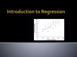
Introduction to Regression Lecture 2.1. Review of Lecture 1.1 Correlation Pitfalls with Regression and Correlation Introducing Multiple Linear Regression Job times case study Stamp sales case study Homework. Review of Lecture 1.1. Scatter plot of US mail handling data, exceptions deleted.

E N D
Introduction to RegressionLecture 2.1 • Review of Lecture 1.1 • Correlation • Pitfalls with Regression and Correlation • Introducing Multiple Linear Regression • Job times case study • Stamp sales case study • Homework Diploma in Statistics Introduction to Regression
Review of Lecture 1.1 Scatter plot of US mail handling data,exceptions deleted Diploma in Statistics Introduction to Regression
Always look ar your data! "Although regression can be done without ever looking at a scatter plot, that is the statistical equivalent of flying blind" Amy Lap Mui Choi, JF MSISS, 1993/94. "Decision-making under risk is when you know what will probably happen and decision-making under uncertainty is when you probably know what will happen." Anon., JF MSISS 1995/96 Diploma in Statistics Introduction to Regression
Simple linear regression modelwith Normal model for chance variation Y = α + βX + Diploma in Statistics Introduction to Regression
The prediction formula Prediction equation: Prediction equation allowing for chance variation: Diploma in Statistics Introduction to Regression
Homework Use the prediction formula to predict the extra manpower requirement during Christmas period, based on the experience of Period 7, Fiscal 1963, when Y was 1,070 and X was 270. Compare with actual. Comment. Diploma in Statistics Introduction to Regression
Application 1Confidence interval for marginal change Recall confidence interval for m: or Confidence interval for b: Small sample: Diploma in Statistics Introduction to Regression
Diploma in Statistics Introduction to Regression
Application 2Testing the statistical significance of the intercept Formal test: H0: a = 0 Test statistic: Critical value: 2 (or t21, .05 = 2.08) Calculated value: 0.848 Comparison: Z < 2 (or t < 2.08) Conclusion: Accept H0 Diploma in Statistics Introduction to Regression
Testing the statistical significance of the intercept Informal test: is less than its standard error, Draw a picture! Diploma in Statistics Introduction to Regression
More on Minitab results Regression Analysis: Manhours versus Volume The regression equation is Manhours = 50.4 + 3.35 Volume Predictor Coef SE Coef T P Constant 50.44 59.46 0.85 0.406 Volume 3.3454 0.3401 9.84 0.000 S = 18.9300 Diploma in Statistics Introduction to Regression
Homework In a study of a wholesaler's distribution costs, undertaken with a view to cost control, the volume of goods handled and the overall costs were recorded for one month in each of ten depots in a distribution network. The results are presented in the following table. Diploma in Statistics Introduction to Regression
Homework The simple linear regression of costs (Y) on volume (X) was calculated, and resulted in the following numerical summary. Regression Analysis: Costs versus Volume The regression equation is Costs = 2.98 + 0.332 Volume Predictor Coef SE Coef T P Constant 2.982 1.646 1.81 0.108 Volume 0.33174 0.03182 10.42 0.000 S = 0.667603 Diploma in Statistics Introduction to Regression
Homework (i) Draw a scatter plot for these data. Comment. Interpret the numerical summary in context. (ii) Calculate a prediction interval for costs next month when Volume in Depot 1 is planned to be £40,000, and Volume in Depot 2 is planned to be £51,000. (iii) Next month, when the two depots recorded volumes of £40,000 and £51,000 as planned, costs were £1,700 and £2,300 respectively. Comment on each case. Illustrate with an enhancement of your scatter plot. Diploma in Statistics Introduction to Regression
Homework Solution (i) There appears to be a strong positive relationship between Costs and Volume. Diploma in Statistics Introduction to Regression
Homework Solution (i) Costs increase approximately linearly with Volume, by around £33.20 for every £1,000 increase in Volume, from a base of around £300. (Costs = 2.98 + 0.332 Volume) The cost for a given volume is subject to chance variation with a standard deviation of around £67. (S = 0.667603) Diploma in Statistics Introduction to Regression
Homework Solution (ii) Volume = £40,000, Costs (£1,491 , £1,759) Volume = £51,000, Costs (£1,857 , £2,124) (iii) £1,700 is within the corresponding prediction interval, satisfactory. £2,300 is outside the corresponding prediction interval, too high. An investigation is needed. Illustrate Diploma in Statistics Introduction to Regression
More precise formulas Confidence interval for mean response: Prediction interval for next response: (ii) Volume = £40,000, Costs (£1,444 , £1,807) Volume = £51,000, Costs (£1,829 , £2,151) Diploma in Statistics Introduction to Regression
Standard error • of prediction • of estimation Ref: "The Standard Error of Prediction" Extra Notes folder in mstuart/get or Diploma webpage Diploma in Statistics Introduction to Regression
Homework Solution Diploma in Statistics Introduction to Regression
2. Correlation • The correlation coefficient formula • r and reduction of prediction error • Positive and negative correlation • Perfect correlation • Conventional interpretations of r Diploma in Statistics Introduction to Regression
The correlation coefficient formula Recall equivalently, Diploma in Statistics Introduction to Regression
Scatter plot showing zero correlation Diploma in Statistics Introduction to Regression
Correlation r = 0.1 to r = 0.9 Data Desk Diploma in Statistics Introduction to Regression
r and reduction in prediction error Diploma in Statistics Introduction to Regression
r and reduction in prediction error Diploma in Statistics Introduction to Regression
Positive and negative correlation Diploma in Statistics Introduction to Regression
Perfect correlation, positive and negative Diploma in Statistics Introduction to Regression
Conventional interpretations of r Science / Engineering: r > 0.9 is "interesting" Econometrics: r > 0.7 is "interesting", otherwise, r > 0.5 is "interesting" Sociology: r > 0.3 is "interesting" Recommendation: compare s to SY Diploma in Statistics Introduction to Regression
3. Pitfalls with regression and correlation Diploma in Statistics Introduction to Regression
Anscombe's data summary Diploma in Statistics Introduction to Regression
Anscombe's scatter plots Diploma in Statistics Introduction to Regression
Homework The shelf life of packaged foods depends on many factors. Dry cereal (such as corn flakes) is considered to be a moisture-sensitive product, with the shelf life determined primarily by moisture. In a study of the shelf life of one brand of cereal, packets of cereal were stored in controlled conditions (23°C and 50% relative humidity) for a range of times, and moisture content was measured. The results were as follows. Draw a scatter diagram. Comment. What action is suggested? Why? Diploma in Statistics Introduction to Regression
Following appropriate action, the following regression was computed. The regression equation is Moisture Content = 2.86 + 0.0417 Storage Time Predictor Coef SE Coef T P Constant 2.86122 0.02488 115.01 0.000 Storage Time 0.041660 0.001177 35.40 0.000 S = 0.0493475 Calculate a 95% confidence interval for the daily change in moisture content; show details. Diploma in Statistics Introduction to Regression
Was the action you suggested on studying the scatter diagram in part (a) justified? Explain. Predict the moisture content of a packet of cereal stored under these conditions for 3 weeks; calculate a prediction interval. What would be the effect on your interval of not taking the action you suggested on studying the scatter diagram? Why? Taste tests indicate that this brand of cereal is unacceptably soggy when the moisture content exceeds 4. Based on your prediction interval, do you think that a box of cereal that has been on the shelf for 3 weeks will be acceptable? Explain. What about 4 weeks? 5 weeks? What is acceptable? Diploma in Statistics Introduction to Regression
Reading SA Sections 6.4, 6.5 Diploma in Statistics Introduction to Regression
4 Introducing Multiple Linear Regression • SLR explaining variation in Y in terms of variation in X • MLR explaining variation in Y in terms of variation in several X 's Diploma in Statistics Introduction to Regression
Example 1What determines the taste of mature cheese? • X1 = Acetic Acid • X2 = Hydrogen Sulphide • X3 = Lactic Acid • Y = Taste Score Diploma in Statistics Introduction to Regression
Example 2Explaining crime rates Variable Description M percentage of males aged 14–24 So indicator variable for a southern state Ed mean years of schooling Po1 police expenditure in 1960 Po2 police expenditure in 1959 LF labour force participation rate M.F number of males per 1000 females Pop state population NW number of nonwhites per 1000 people U1 unemployment rate of urban males 14–24 U2 unemployment rate of urban males 35–39 GDP gross domestic product per head Ineq income inequality Prob probability of imprisonment Time average time served in state prisons Crime rate of crimes in a particular category per head of population Diploma in Statistics Introduction to Regression
Example 3Estimating tree volume / timber yield For a sample of 31 black cherry trees in the Allegheny National Forest, Pennsylvania, measure • Y = volume (cubic feet), • X1 = height (feet) • X2 = diameter (inches) (at 54 inches above ground Diploma in Statistics Introduction to Regression
Example 4The Stamp Sales Case Study The problem • January 1984, An Post established • New business plan; sales forecasts required • Historical sales data available bring in a consultant! Diploma in Statistics Introduction to Regression
Example 5A production prediction problem • The problem • The data • Initial data analysis • dotplots • lineplots (time series plots) • scatterplot matrix • Model fitting / estimation • Model criticism • Application Diploma in Statistics Introduction to Regression
Erie Metal Products: The problem Metal products fabrication: customers order varying quantities of products of varying complexity; customers demand accurate and precise order delivery times. Diploma in Statistics Introduction to Regression
Rear view Stephan Clark Metal Products A specially designed cabinet Diploma in Statistics Introduction to Regression
Another view Stephan Clark Metal Products Instrument casing Diploma in Statistics Introduction to Regression
Lockers Stephan Clark Metal Products Instrument casing; oblique view Diploma in Statistics Introduction to Regression
Stephan Clark Metal Products • "One customer is an international manufacturer of petrochemical equipment." • "Stephen Clark supplies painted metalwork components, panels and fabrications, which are used throughout the customer's product range." • "Stephen Clark plays an important part in them being able to cope with frequent scheduling changes." • "Through careful program management, we are able to offer excellent flexibility of supply, delivering finished product against weekly call-offs." Diploma in Statistics Introduction to Regression
Erie Metal Products: The data Diploma in Statistics Introduction to Regression
The variables • Response: • Jobtime, time (hours) to complete an order • Explanatory: • Units, the number of units ordered • Operations per Unit, the number of operations involved in manufacturing a unit, • Rushed, indicator of "rushed" priority status • Total Operations Units × Operations per Unit Diploma in Statistics Introduction to Regression
Initial data analysis, dotplots Diploma in Statistics Introduction to Regression