Download
1 / 51
510 likes | 685 Views
GEOLOGY 415/515: TECTONIC GEODESY C. Rubin, Central Washington University. Introduction Earthquakes: fundamental concepts & focal mechanisms Earthquakes: magnitude, earthquake cycle Tectonic geodesy Strike-slip faults Normal faults Subduction zones (Megathrust earthquakes)

E N D
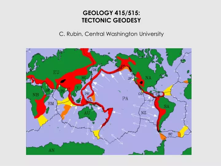
GEOLOGY 415/515: TECTONIC GEODESY C. Rubin, Central Washington University
Introduction Earthquakes: fundamental concepts & focal mechanisms Earthquakes: magnitude, earthquake cycle Tectonic geodesy Strike-slip faults Normal faults Subduction zones (Megathrust earthquakes) Thrust/Reverse faults Plate interiors Earthquake recurrence & hazards
Shaded ellipses depict typical ranges for classes of processes. Hachured boundaries indicate the present range of various techniques for making geodetic measurements. EDM: electronic distance meter GPS: global positioning system OB: observation SLR: satellite laser ranging VLBI: very long baseline interferometry. Modified after Minster et al. (1990).
Displacement at three intervals, beginning with t0 is illustrated. A. Fault zone is very weak and is creeping so that all motion occurs directly along fault. B. Fault zone is relatively strong and strain is distributed across broad zone on either side of the fault.
C. Some creep occurs on the fault, and rigid block rotations occur on either side of the fault, taking up the additional motion. D. Schematic results from an alignment array along a creeping fault that is displaced about 80 mm in 20 years. Modified after Sylvester (1986).
GPS GEODESY Repeated measurements that locate of certain fixed reference points on the Earth's surface. Fixed points are marked by metal disks set into concrete casings (called bench-marks) or very stable structures called monuments. The Earth’s surface can move up, down and sideways - the reference point includes a vertical position and horizontal position. The horizontal position of a reference point is described by its latitude (north-south position) and longitude (east-west position). The vertical position of a reference point is described by its height above or below mean sea level.
GPS GEODESY Global mean sea level is complicated since the Earth's mass is not uniformly distributed within an elliptical shell. Areas with greater mass have a stronger gravitational attraction than areas with less mass, and these differences cause differences in actual mean sea level on the Earth's surface. To account for these differences, geodesists imagine a three-dimensional surface so that the Earth's gravitational attraction is the same at every point on the surface. This surface is called the geoid, and is a closer approximation to global mean sea level than the ellipsoid.
Global Sea Level Gravity anomaly map from the NASA GRACE (Gravity Recovery And Climate Change).
GPS GEODESY • The original design of the GPS space segment, with 24 GPS satellites (4 satellites in each of 6 orbits), showing the evolution of the number of visible satellites from a fixed point (45ºN) on earth (considering "visibility" as having direct line of sight). • Each GPS satellite continuously broadcasts a Navigation Message giving: • SATELLITE CLOCK AND ITS RELATIONSHIP TO GPS SYSTEM TIME • EPHEMERIS - GIVING THE SATELLITE'S OWN PRECISE ORBIT • COARSE ORBIT AND STATUS INFORMATION FOR EACH satellite in the constellation, an ionospheric model, and information to relate GPS derived time to Coordinated Universal Time (UTC). Each satellite transmits its navigation message with at least two distinct spread spectrum codes: the Coarse / Acquisition (C/A) code, which is freely available to the public, and the Precise (P) code, which is usually encrypted.
GPS GEODESY A GPS receiver computes the distance to a satellites based onamount of time required for a radio signal from the satellite to reach the receiver. The satellites and receivers both contain accurate clocks (the satellites contain an atomic clock that is much more accurate than the receivers' clock, however), The receiver calculates the time difference between the two signals, and then converts this to a distance measurement. Four satellites are typically used to determine the three-dimensional position of a location on Earth. 4 unknowns: x, y, z coordinates and time
GPS ERRORS Atmospheric effects Inconsistencies of atmospheric conditions affect the speed of the GPS signals as they pass through the Earth's atmosphere, especially the ionosphere Multipath effects GPS signals can also be affected by multipath issues, where the radio signals reflect off surrounding terrain; buildings, canyon walls, hard ground, etc. These delayed signals can cause inaccuracy.
GPS ERRORS Ephemeris and clock errors The ephemeris data is transmitted every 30 seconds, the information itself may be up to two hours old. Data up to four hours old is considered valid for calculating positions, but may not indicate the satellites actual position. The satellite's atomic clocks experience noise and clock drift errors. The navigation message contains corrections for these errors and estimates of the accuracy of the atomic clock, however they are based on observations and may not indicate the clock's current state.
Displacement at three intervals, beginning with t0 is illustrated. A. Fault zone is very weak and is creeping so that all motion occurs directly along fault. B. Fault zone is relatively strong and strain is distributed across broad zone on either side of the fault.
C. Some creep occurs on the fault, and rigid block rotations occur on either side of the fault, taking up the additional motion. D. Schematic results from an alignment array along a creeping fault that is displaced about 80 mm in 20 years. Modified after Sylvester (1986).
V is the rate of relative motion between the two blocks v/V is the fraction of the total motion that is exhibited by any point. The rigidity of the fault (m2) is one-fifth that of the right-hand block (m1). Most of the displacement occurs along the weak fault zone. Note how the relative rigidity of the blocks affects the shape of the displacement within each block. For the highest rigidity (line 5, left-hand block), there is very little deformation within the rigid block . Modified after Lisowski et al. (1991).
Aseismic creep refers to fault slip that does not produce seismic radiation. Both geological and geodetic observations document evidence of creep along many fault segments in California. Fault creep releases elastic strain and reduces the hazard from future earthquakes, making it an important part of seismic hazard estimation.
a. Fault slip versus depth for the complete earthquake cycle, after Tse and Rice [1986]. At each depth, the sum of the co-, post- and inter-seismic slip must equal the geologic displacement. b. Surface displacement across the fault for the co-, post- and inter-seismic parts of the cycle. The near-field surface displacement for both the co- and inter-seismic phases depends on the depth distribution of fault creep during the inter-seismic period.
c. Schematic for interseismic strain accumulation. At shallow depths (0 - 4 km), a velocity strengthening zone occurs along well-developed faults resulting in stable sliding at shallow depth [Marone and Scholz, 1988]. Similarly, there is a velocity strengthening zone at greater depth (> ~12 km). d. Fit of GPS velocity data across the Imperial fault [Lyons et al., 2002] reveals a locked zone between 2.9 and 10 km depth. Velocity strengthening - Why is this present?
Geodetic networks Monterey geodetic network showing triangulation stations in the vicinity of the San Andreas and Calaveras faults. B. Results of trilateration surveys between 1973 and 1989 across the San Andreas fault zone near Monterey Bay. Long-term slip rates across the San Andreas region are about 35 mm/yr in this area.
About 15 mm/yr of North America-Pacific relative plate motion is accommodated on other faults beyond the surveyed area. The San Andreas and the Calaveras faults are clearly marked by abrupt changes in relative velocity. These discontinuities show that most of the relative motion across this 80-km-wide zone is accommodated by slip on these two faults. Creep or locked fault based on geodetic data?
Little deformation occurs in the bounding blocks. • Over a span of 16 years, the total motion across the profile is averages about 35 mm/yr • Most of the expected plate motion is accounted for by the measured velocities. Abrupt change of velocity across fault – creeping or freely slipping fault
Geodetic networks Triangulation network in the vicinity of the Transverse Ranges of southern California. The Transverse Range data (1973-1989) shows no differential displacement across the San Andreas fault. Creep or locked fault based on geodetic data?
No differential displacement across the San Andreas fault, Interpreted as a locked fault in this region. Instead, strain is occurring across the entire surveyed zone. How much strain is accumulating across the fault zone?
Less than 25 mm/yr of relative plate motion is accommodated by displacements along the profile. • This indicates that considerable strain due to Pacific-North American relative plate motion occurs well beyond the San Andreas fault zone.
Himalaya front - Nepal Relative uplift rates are calculated along a 250-km-long spirit-leveling line (B) oriented approximately perpendicular to the Himalayan Range in central Nepal. The profile is fixed at its southern end, and errors become cumulatively larger to the north.
The southernmost peak of uplift (~2 mm/yr) is interpreted as a response to a growing anticline within the foreland. No distinct topographic signature is associated with this deformation, probably due to ready erosion of the uplifted strata.
The leveling line through the Lesser Himalaya shows uplift spatially associated with the Main Boundary Thrust and subsidence in the intermontane Kathmandu region. Uplift within the Greater Himalaya occurs at the highest rates (~6 mm/yr) and is associated with high topography.
Finite-element modelling of deformation of elastic crust (bottom panel) suggests that strain above and south of a crustal ramp separating the Indian and Asian plates could generate the observed pattern of uplift. Modified after Jackson and Bilham (1994a).
Comparison of leveling-line data and deformed river terraces along a growing fold. Coseismic deformation from the 1983 Coalinga earthquake (M = 6.5) from leveling-line data along the center of the anticline (line, inset).
B. Deformed terrace profile surveyed near the nose of the same anticline (line 1, inset). Similar deformation patterns are displayed by both data set. The long-term pattern of terrace deformation could result from the accumulation of deformation similar to that caused by the 1983 Coalinga earthquake. Modified after King and Stein (1983).
The magnitude of warping is calculated by subtracting the estimated undisturbed terrace profile from the observed profile. Modified after King and Stein (1983).
Plate tectonic boundary geodetic changes CONVERGENCE - ALEUTIAN TRENCH 54 mm/yr CONVERGENCE - CASCADIA 33-41 mm/yr PACIFIC wrt NORTH AMERICA pole STRIKE SLIP - SAN ANDREAS EXTENSION - GULF OF CALIFORNIA
1989 LOMA PRIETA, CALIFORNIA EARTHQUAKE MAGNITUDE 7.1 ON THE SAN ANDREAS Davidson et al
GPS & EQ Cycle Geodetic measurements of crustal movements in California provide critical observations for understanding earthquakes. Almost a century ago, Read (1910) analyzed geodetic measurements acquired before and after the 1906 San Francisco Earthquake to establish his “elastic rebound” theory (Figure 1).
GPS & EQ Cycle The theory proposes a two stage model of crustal deformation: Elastic behavior in between earthquakes (interseismic) and Fault rupture (coseismic) during earthquakes. The elastic rebound theory expanded into a four stage conceptual model, known as the “the earthquake deformation cycle”. The two additional stages are pre- and post-seismic (afterslip) deformation, occurring short time before and after the large earthquake, respectively.
GPS Velocity field - SAF • The velocity vectors with respect to the Stable North America reference frame • Southwestward magnitude increase. • In this reference frame, crustal movements in eastern US (east of the Colorado Plateau) are zero and increase in tectonically active areas, such as western US.
GPS & EQ Cycle A subset of the GPS velocity field in Central California showing velocity variations across the San Andreas Fault. The velocities are shown in the stable North America reference frame.
GPS & EQ Cycle Map of the San Francisco Bay area in a Pacific Plate-Sierra Nevada block projection with GPS Velocities from 1994-2003 relative to station LUTZ in the Bay Block (yellow square).
GPS Velocity field SAF • The region affected by postseismic deformation following the Loma Prieta earthquake. • To avoid "contamination" of the regional deformation pattern by transient processes, data before 1994 is not included. • The southern Bay Area exhibits mostly fault-parallel right-lateral motion, with no indication of the fault-normal compression observed in the Foothills thrust belt immediately after the Loma Prieta Earthquake (Bürgmann, 1997).
GPS & EQ Cycle Creep along the Hayward fault allows the Bay block to slide past the East Bay Hills block Only minimal internal deformation and strain accumulation within either block. Deformation near the Hayward fault. Velocities relative to LUTZ on the Bay block.
Fixed Pacific plate • Most displacement east of SAF are parallel to fault • West of SAF, between SB and LA, displacement is accommodated by other faults (thrust and reverse) • Variability of motions = differential rotation of blocks • Plate boundary not just concentrated along SAF
Given the background noise in the observations, it is only with continuous GPS readings that this trend (1.1 mm/day) is observable. Modified after Bock et al. (1993).
Despite the typical day-to-day variability of 5-15 mm, very precise positions are defined using multiple days of readings. An abrupt coseismic offset of 44 mm occurred during the 1991 Landers earthquake. Post-seismic slip of 22 mm that occurred during the few weeks following the EQ (right panel). Given the background noise in the observations, it is only with continuous GPS readings that this trend (1.1 mm/day) is observable. Modified after Bock et al. (1993).
Radar SAR interferogram of ground displacement associated with the Landers Mw 7.3 earthquake of June, 1992. Each fringe represents 28 mm of displacement and at least 20 fringes are visible near the fault (equal to 560 mm of displacement). Coherence is lost as the ground rupture is approached, probably because the displacement gradient is greater than 28 mm/pixel. Massonnet et al. (1993).
Note the broad, asymmetric deformation in an east-west direction covering >75 km and the abrupt termination of major deformation near the ends of the fault. The detailed deformation patterns seen here can be used to constrain models of surface displacement due to the Landers rupture.
B. Modeled interferogram pattern based on eight fault segments rupturing along vertical planes in an elastic half-space. The excellent match between the observed and modeled results indicates that a simple half-space model models the observed deformation pattern. Modified after Massonnet et al. (1993).
Mt Etna interferogram X-band (SIR-C/X-SAR mission)