Download
1 / 56
560 likes | 755 Views
Lecture 1 : Measurements, Statistics, Probability, and Data Display. Karen Bandeen -Roche, PhD Department of Biostatistics Johns Hopkins University. July 11, 2011. Introduction to Statistical Measurement and Modeling. What is statistics?. The study of … ( i .) … populations

E N D
Lecture 1: Measurements, Statistics, Probability, and Data Display Karen Bandeen-Roche, PhD Department of Biostatistics Johns Hopkins University July 11, 2011 Introduction to Statistical Measurement and Modeling
What is statistics? The study of … (i.) … populations (ii.) …variation (iii.) … methods of the reduction of data. “The original meaning of the word … suggests that it was the study of populations of human beings living in political union.” Sir R. A. Fisher
What is statistics? • “… Statistical Science [is] the particular aspect of human progress which gives the 20th century its special character…. It is to the statistician that the present age turns for what is most essential in all its more important activities.” Sir R. A. Fisher
What is statistics?Less complimentary views • “Science is difficult. You need mathematics and statistics, which is dull like learning a language.”Richard Gregory • “There are three kinds of lies: lies, damned lies and statistics.” Mark Twain, quoting Disraeli
What is statistics? • Statistics in concerned with METHODS for COLLECTING & DESCRIBING DATA and then for ASSESSING STRENGTH OF EVIDENCE in DATA FOR/AGAINST SCIENTIFIC IDEAS!” Scott L. Zeger
What is statistics? • the art and science of gathering, analyzing, and making inferences from data.”Encyclopaedia Britannica Poetry Music Mathematics Physics Statistics
What is biostatistics? • The science of learning from biomedical data involving appreciable variability or uncertainty. Amalgam
Data examples • Osteoporosis screening • Importance: Osteoporosis afflicts millions of older adults (particularly women) worldwide • Lowers quality of life, heightens risk of falls etc. • Scientific question: Can we detect osteoporosis earlier and more safely? • Method: ultrasound versus dual photon absorptiometry (DPA) tried out on 42 older women • Implications: Treatment to slow / prevent onset
Data examples • Temperature modeling • Importance: Climate change is suspected. Heat waves, increased particle pollution, etc. may harm health. • Scientific question: Can we accurately and precisely model geographic variation in temperature? • Method: Maximum January-average temperature over 30 years in 62 United States cites • Implications: Valid temperature models can support future policy planning
United States temperature map http://green-enb150.blogspot.com/2011/01/isorhythmic-map-united-states-weather.html
Modeling geographical variation:Latitude and Longitude http://www.enchantedlearning.com/usa/activity/latlong/
Data examples • Boxing and neurological injury • Importance: (1) Boxing and sources of brain jarring may cause neurological harm. (2) In ~1986 the IOC considered replacing Olympic boxing with golf. • Scientific question: Does amateur boxing lead to decline in neurological performance? • Method: “Longitudinal” study of 593 amateur boxers • Implications: Prevention for brain injury from subconcussive blows.
Data examples • Temperature modeling • Importance: Climate change is suspected. Heat waves, increased particle pollution, etc. may harm health. • Scientific question: Can we accurately and precisely model geographic variation in temperature? • Implications: Valid temperature models can support future policy planning
Course objectives • Demonstrate familiarity with statistical tools for characterizing population measurement properties • Distinguish procedures for deriving estimates from data and making associated scientific inferences • Describe “association” and describe its importance in scientific discovery • Understand, apply and interpret findings from • methods of data display • standard statistical regression models • standard statistical measurement models • Appreciate roles of statistics in health science
Basic paradigm of statistics • We wish to learn about populations • All about which we wish to make an inference • “True” experimental outcomes and their mechanisms • We do this by studying samples • Asubsetof a given population • “Represents” the population • Sample features are used to inferpopulation features • Method of obtaining the sample is important • Simple random sample: All population elements / outcomes have equal probability of inclusion
Basic paradigm of statistics Probability Observed Value for a Representative Sample Truth for Population Statistical inference
Tools for description • Populations • Probability • Parameters • Values, distributions • Hypotheses • Models • Samples • Probability • Statistics / Estimates • Data displays • Statistical tests • Analyses
Probability • Way for characterizing random experiments • Experiments whose outcome is not determined beforehand • Sample space: Ω := {all possible outcomes} • Event = A ⊆ Ω := collection of some outcomes • Probability = “measure” on Ω • Our course: measure of relative frequency of occurrence • “Bayesian”: measure of relative belief in occurrence
Probability measures • Satisfy following axioms: i) P{Ω} = 1: reads "probability of Ω" ii) 0 ≤ P{A} ≤ 1 for each A > 0 = “can’t happen”; 1 = “must happen” iii) Given disjoint events {Ak}, P{ } = Σ P{Ak} > “disjoint” = “mutually exclusive”; no two can happen at the same time
Random variable (RV) • A function which assigns numbers to outcomes of a random experiment - X:Ω → ℝ • Measurements • Support:= SX = range of RV X • Two fundamental types of measurements • Discrete: SX is countable (“gaps” in possible values) • Binary: Two possible outcomes • Continuous: SX is an interval in ℝ • “No gaps” in values
Random variable (RV) • Example 1: X = number of heads in two fair coin tosses • SX = • Example 2: Draw one of your names out of a hat. X=age (in years) of the person whose name I draw. • SX = • Mass function: {0,1,2}
Probability distributions • Heuristic: Summarizes possible values of a random variable and the probabilities with which each occurs • Discrete X: Probability mass function = list exactly as the heuristic: p:x → P(X=x) • Example = 2 fair coin tosses: • P{HH} = P{HT} = P{TH} = P{TT} = ¼ • Mass function: xp(x) = P(X=x) 0 ¼ 1 ½ 2 ¼ y {0,1,2} 0
Cumulative probability distributions • F: x → P(X ≤ x) = cumulative distribution function CDF • Discrete X: Probability mass function = list exactly as the heuristic • Example = 2 fair coin tosses:
Cumulative probability distributions • Example = 2 fair coin tosses: • Notice: p(x) recovered as differences in values of F(x) • Suppose x1≤ x2≤ … and SX = {x1, x2, …} • p(xi) = F(xi) - F(xi-1), each i (define x0= -∞ and F(x0)=0)
Cumulative probability distributions • Draw one of your names out of a hat. X=age (in years) of the person whose name I draw
What about continuous RVs? • Can we list the possible values of a random variable and the probabilities with which each occurs? • NO. If SX is uncountable, we can’t list the values! • The CDF is the fundamental distributional quantity • F(x) = P{X≤x}, with F(x) satisfying i) a ≤ b ⇒ F(a) ≤ F(b); ii) lim (b→∞) F(b) = 1; iii) lim (b→-∞) F(b) = 0; iv) lim (bn ↓ b) F(bn) = b v) P{a<X≤b} = F(b) - F(a)
Two continuous CDFs • “Normal” • “Exponential”
Mass function analog: Density • Defined when F is differentiable everywhere (“absolutely continuous”) • Thedensity f(x) is defined as • lim(ε↓0) P{X є [x-ε/2,x+ε/2]}/ε • = lim(ε↓0) [F(x+ε/2)-F(x-ε/2)]/ε • = d/dy F(y) |y=x • Properties • i) f ≥ 0 • ii) P{a≤X≤b} = ∫ab f(x)dx • iii) P{XεA} = ∫A f(x)dx • iv) ∫-∞∞ f(x)dx = 1
Two densities • “Normal” • “Exponential
Probability model parameters • Fundamental distributional quantities: • Location: ‘central’ value(s) • Spread: variability • Shape: symmetric versus skewed, etc.
Location and spread (Different Locations) (Different Spreads)
Probability model parameters • Location • Mean: E[X] = ∫ xdF(x) = µ • Discrete FV: E[X] = ΣxεSX xp(x) • Continuous case: E[X] = ∫ xf(x)dx • Linearity property: E[a+bX] = a + bE[X] • Physical interpretation: Center of mass
Probability model parameters • Location • Median • Heuristic: Value so that ½ of probability weight above, ½ below • Definition: median is m such that F(m) ≥ 1/2, P{X≥m} ≥ ½ • Quantile ("more generally"...) • Definition: Q(p) = q: FX(q) ≥ p, P{X≥q} ≥ 1-p • Median = Q(1/2)
Probability model parameters • Spread • Variance: Var[X] = ∫(x-E[X])2dF(x) = σ2 • Shortcut formula: E[X2]-(E[X])2 • Var[a+bX] = b2Var[X] • Physical interpretation: Moment of inertia • Standard deviation: SD[X] = σ = √(Var[X]) • Interquartile range (IQR) = Q(.75) - Q(.25)
Pause / Recapitulation • We learn about populations through representative samples • Probability provides a way to characterize populations • Possibly unseen (models, hypotheses) • Random experiment mechanisms • We will now turn to the characterization of samples • Formal: probability • Informal: exploratory data analysis (EDA)
Describing samples • Empirical CDF • Given data X1,...,Xn, Fn(x) = {#Xi's ≤ x}/n • Define indicator 1{A}:= 1 if A true = 0 if A false • ECDF = Fn = (1/n)Σ 1{Xi≤x} = probability (proportion) of values ≤ x in sample • Notice is real CDF with correct properties • Mass function px = 1/n if x ε {X1,...,Xn}; = 0 otherwise.
Sample statistics • Statistic = Function of data • As defined in probability section, with F=Fn • Mean = = ∫ xdFn(x) = (1/n) Σ Xi. • Variance = s2 = • Standard deviation = s
Sample statistics - Percentiles • “Order statistics” (sorted values): • X(1) = min(X1,...,Xn) • X(n) = max(X1,...,Xn) • X(j) = jth largest value, etc. • Median = mn = {x:Fn(x)≥1/2} and {x:PFn{X≥x}≥1/2 = X((n+1)/2) = middle if n odd; = [X(n/2)+X(n/2+1)]/2 = mean of middle two if n even • Quantile Qn(p) = {x:Fn(x)≥p} and {x:PFn{X≥x}≥1-p} • Outlier = data value "far" from bulk of data
Describing samples - Plots • Stem and leaf plot: Easy “density” display • Steps • Split into leading digits, trailing digits • Stems: Write down all possible leading digits in order, including “might have occurred's” • Leaves: For each data value, write down first trailing digit by appropriate value (one leaf per datum). • Issue: # stems • Chiefly science • Rules of thumb: root-n, 1+3.2log10n
Describing samples - Plots • Boxplot • Draw box whose "ends" are Q(1/4) and Q(3/4) • Draw line through box at median • Boxplot criterion for "outlier": beyond "inner fences" = hinges +/- 1.5*IQR • Draw lines ("Whiskers") from ends of box to last points inside inner fences • Show all outliers individually • Note: perhaps greatest use = with multiple batches
Introduction: Statistical Modeling • Statistical models: systematic + random • Probability modeling involves random part • Often a few parameters “Θ” left to be estimated by data • Scientific questions are expressed in terms of Θ • Model is tool / lens / function for investigating scientific questions • "Right" versus "wrong" misguided • Better: “effective” versus “not effective”
Modeling: Parametric Distributions • Exponential distribution F(x) = 1-e-λx if x ≥ 0 = 0 otherwise • Model parameter: λ = rate • E[X] = 1/λ • Var[X] = 1/λ2 • Uses • Time-to-event data • “Memoryless”
Modeling: Parametric Distributions • Normal distribution f(x) = on support SX = (-∞, ∞). • Distribution function has no closed form: • F(x) := ∫-∞x f(t)dt, f given above • F(x) tabulated, available from software packages • Model parameters: μ=mean; σ2=variance
Normal distribution • Characteristics a) f(x) is symmetric about μ b) P{μ-σ≤X≤μ+σ} ≈ .68 c) P{μ-2σ≤X≤μ+2σ} ≈ .95 • Why is the normal distribution so popular? a) If X distributed as (“~”) Normal with parameters (μ,σ) then (X-μ)/σ = “Z” ~ Normal (μ=0,σ=1) b) Central limit theorem: Distributions of sample means converge to normal as n →∞