Download
1 / 35
350 likes | 446 Views
Randomness in Computation and Communication. Part 1: Randomized algorithms. Lap Chi Lau CSE CUHK. Making Decision. Flip a coin. Making Decision. Flip a coin!. An algorithm which flip coins is called a randomized algorithm. Why Randomness?.

E N D
Randomness in Computation and Communication Part 1: Randomized algorithms Lap Chi Lau CSE CUHK
Making Decision Flip a coin.
Making Decision Flip a coin! An algorithm which flip coins is called a randomized algorithm.
Why Randomness? Making good decisions could be complicated and expensive. A randomized algorithm is often simpler and faster. • Minimum spanning trees A linear time randomized algorithm, but no known linear time deterministic algorithm. • Primality testing A randomized polynomial time algorithm, but it takes thirty years to find a deterministic one. • Volume estimation of a convex body A randomized polynomial time approximation algorithm, but no known deterministic polynomial time approximation algorithm.
Minimum Cut A cut is a set of edges whose removal disconnects the graph. Minimum cut: Given an undirected multi-graph G with n vertices, find a cut of minimum cardinality (a min-cut).
Minimum Cut A cut is a set of edges whose removal disconnects the graph. Minimum cut: Given an undirected multi-graph G with n vertices, find a cut of minimum cardinality (a min-cut). A minimum s-t cut can be solved in polynomial time by a max-flow algorithm. t s Minimum s-t cut = maximum number of edge-disjoint s-t paths
Minimum Cut Naive: To compute the (global) min-cut, an algorithm is to compute minimum s-t cuts for all pairs of s and t, and take the minimum one. Running time: O(n2 · max-flow) = O(n3 · m) Observation: fix s and consider minimum s-t cuts for t. Running time: O(n · max-flow) = O(n2 · m) [Nagamochi-Ibaraki 92,Stoer-Wagner 97] O(nm + n2 log n) new ideas that lead to faster randomized algorithms
Edge Contraction 5 5 1 4 4 3 3 2 1,2 Contraction of an edge e = (u,v): Merge u and v into a single vertex “uv”. For any edge (w,u) or (w,v), this edge becomes (w,“uv”) in the resulting graph. Delete any edge which becomes a “self-loop”, i.e. an edge of the form (v,v).
Edge Contraction 5 5 1 4 4 3 3 2 1,2 Observation: an edge contraction would not decrease the min-cut size. This is because every cut in the graph at any intermediate stage is a cut in the original graph.
A Randomized Algorithm Running time: Each iteration takes O(n) time. Each iteration has one fewer vertex. So, there are at most n iteration. Total running time O(n2). • Algorithm Contract: • Input: A multigraph G=(V,E) • Output: A cut C • H <- G. • while H has more than 2 vertices do • 2.1 choose an edge (x,y) uniformly at random from the edges in H. • 2.2 H <- H/(x,y). (contract the edge (x,y)) • 3. C <- the set of vertices corresponding to one of the two meta-vertices in H.
Analysis Obviously, this algorithm will not always work. How should we analyze the success probability? Let C be a minimum cut, and E(C) be the edges crossing C. Claim 1: C is produced as output if and only if none of the edges in E(C) is contracted by the algorithm. So, we want to estimate the probability that an edge in E(C) is picked. What is this probability?
Analysis Let k be the number of edges in E(C). How many edges are there in the initial graph? Claim 2: The graph has at least nk/2 edges. Because each vertex has degree at least k. So, the probability that an edge in E(C) is picked at the first iteration is at most 2/n.
Analysis In the i-th iteration, there are n-i+1 vertices in the graph. Observation: an edge contraction would not decrease the min-cut size. So the min-cut still has at least k edges. Hence there are at least (n-i+1)k/2 edges in the i-th iteration. The probability that an edge in E(C) is picked is at most 2/(n-i+1).
Analysis So, the probability that a particular min-cut is output by Algorithm Contract with probability at least Ω(n-2).
Boosting the Probability To boost the probability, we repeat the algorithm for n2log(n) times. What is the probability that it still fails to find a min-cut? So, high probability to find a min-cut in O(n4log(n)) time.
Reflecting This algorithm was proposed by Karger in 1993. It is a simpler algorithm for minimum cut, but is slower and could make mistakes… New way of thinking, leading to a revolution. We first present the improvement by Karger and Stein in 1993.
Ideas to an Improved Algorithm Key: The probability that an edge in E(C) is picked is at most 2/(n-i+1). Observation: at early iterations, it is not very likely that the algorithm fails. Idea: “share” the random choices at the beginning! In the previous algorithm, we boost the probability by running the Algorithm Contract (from scratch) independently many times. G n contractions n2 leaves
Ideas to an Improved Algorithm Idea: “share” the random choices at the beginning! G G n/2 contractions n contractions n/4 contractions ……………… n/8 contractions n2 leaves n2 leaves Previous algorithm. New algorithm. log(n) levels
A Fast Randomized Algorithm • Algorithm FastCut: • Input: A multigraph G=(V,E) • Output: A cut C • n <- |V|. • if n <= 6, then compute min-cut by brute-force enumeration else • 2.1 t <- (1 + n/√2). • 2.2 Using Algorithm Contract, perform two independent contraction sequences to obtain graphs H1 and H2 each with t vertices. • 2.3 Recursively compute min-cuts in each of H1 and H2. • 2.4 return the smaller of the two min-cuts.
A Surprise Theorem 1: Algorithm Fastcut runs in O(n2 log(n)) time. Theorem 2: Algorithm Fastcut succeeds with probability Ω(1/log(n)). By a similar boosting argument, repeating Fastcut for log2(n) times would succeed with high probability. Total running time = O(n2 log3(n))! It is much faster than the best known deterministic algorithm, which has running time O(n3). Min-cut is faster than Max-Flow!
Complexity Theorem 1: Algorithm Fastcut runs in O(n2 log(n)) time. G n/2 contractions n/4 contractions log(n) levels n/8 contractions n2 leaves First level complexity = 2 x (n2/2) = n2. Second level complexity = 4 x (n2/4) = n2. Total time = n2 log(n). The i-th level complexity = 2i x (n2/2i) = n2.
Analysis Theorem 2: Algorithm Fastcut succeeds with probability Ω(1/log(n)). G n/2 contractions n/4 contractions log(n) levels n/8 contractions n2 leaves Claim: for each “branch”, the survive probability is at least ½.
Analysis Theorem 2: Algorithm Fastcut succeeds with probability Ω(1/log(n)). Proof: Let k denote the depth of recursion, and p(k) be a lower bound on the success probability. Solving the recurrence will give:
Remarks Fastcut is fast, simple and cute. Error probability is independent of the problem instance. Combinatorial consequence: # of min cut is O(n2). [Karger 96] Near linear time algorithm for minimum cut, O(m log3n). Open problem 1: deterministic o(mn) min-cut algorithm? Open problem 2: fast randomized min s-t cut algorithm?
Bipartite Matching A matching M is a subset of edges so that every vertex has degree at most one in M. The bipartite matching problem: Find a matching with the maximum number of edges. [Hopcroft-Karp 73] Bipartite matching solved in O(m√n) time.
Edmonds Matrix A perfect matching is a matching in which every vertex is matched. We will present a “fast” randomized algorithm for finding a perfect matching. The algorithm is based on some algebraic techniques. v1 v2 v3 v4 u1 v1 u1 x11 x14 0 0 u2 v2 x22 x23 u2 0 0 u3 v3 u3 x32 x33 0 0 u4 v4 u4 x41 x42 x43 0 Step 1: construct a matrix with one variable for each edge.
Edmonds Matrix Step 2: consider the determinant of the matrix. v1 v2 v3 v4 u1 v1 u1 x11 x14 0 0 u2 v2 x22 x23 u2 0 0 u3 v3 u3 x32 x33 0 0 u4 v4 u4 x41 x42 x43 0 [Edmonds] The determinant is non-zero if and only if there is a perfect matching
Edmonds Matrix Step 2: consider the determinant of the matrix. v1 v2 v3 v4 u1 v1 u1 x11 x14 0 0 u2 v2 x22 x23 u2 0 0 u3 v3 u3 x32 x33 0 0 u4 v4 u4 x41 x42 x43 0 [Edmonds] The determinant is non-zero if and only if there is a perfect matching
Complexity [Edmonds] The determinant is non-zero if and only if there is a perfect matching v1 v2 v3 v4 u1 x11 x14 0 0 x22 x23 u2 0 0 u3 x32 x33 0 0 u4 x41 x42 x43 0 There is no way to compute this determinant efficiently…
Algebraic Algorithm [Edmonds] The determinant is non-zero if and only if there is a perfect matching Step 3 [Lovasz]: pick a large field, substitute random values into the variables. v1 v2 v3 v4 v1 v2 v3 v4 u1 x11 x14 0 0 u1 5 2 0 0 x22 x23 u2 0 0 3 5 u2 0 0 u3 x32 x33 0 0 u3 7 2 0 0 u4 x41 x42 x43 0 u4 1 9 4 0 Step 4: Compute this determinant, say yes if and only if it is nonzero.
Analysis v1 v2 v3 v4 u1 5 2 0 0 3 5 u2 0 0 u3 7 2 0 0 u4 1 9 4 0 If there is no perfect matching, then det(M) must be equal to zero. But if there is a perfect matching, then det(M) may be equal to zero. (due to cancellation) How to analyze the probability of failure?
Analysis v1 v2 v3 v4 u1 5 2 0 0 3 5 u2 0 0 u3 7 2 0 0 u4 1 9 4 0 How to analyze the probability of failure? Problem: if there is a perfect matching, then det(M) may be equal to zero. Observation: det(M) is a degree n multivariate polynomial. (low degree polynomial, not so many roots) [Schwartz Zippel] If the field size is |S|, then failure probability <= n/|S|. So if the field size is large (say n3), then the error probability is very small.
Complexity [Coppersmith Winogrod 90] Determinant can be computed in O(n2.376) time So we can use it to test if there is a perfect matching in the graph. [Mucha Sankowski 04] [Harvey 06] A maximum matching can be constructed in O(n2.376) time Work also for general graph matching, and some other optimization problems.
Remarks Polynomial identify testing is an important problem that can be solved in randomized polynomial time but not known to be solvable in deterministic polynomial time. Red-Black matching: Given a bipartite graph with edges of 2 colors, red and black, decide if there is a perfect matching with exactly k red edges and n-k black edges. Open problem 1: Deterministic polynomial time algorithm for red-black matching? Open problem 2: Weighted matching in O(n2.376) time? Open problem 3: Fast algebraic algorithms for other optimization problems?
Concluding Remarks There are still many basic open problems in this area. • Fast randomized algorithms for minimum s-t cut? • Fast algebraic algorithms for weighted problems? • Fast randomized algorithms for maximum flow? See one interesting recent result in the problem set.