Download
1 / 40
420 likes | 660 Views
Clustering Algorithms. Hierarchical Clustering k -Means Algorithms CURE Algorithm. Methods of Clustering. Hierarchical (Agglomerative) : Initially, each point in cluster by itself. Repeatedly combine the two “nearest” clusters into one. Point Assignment : Maintain a set of clusters.

E N D
Clustering Algorithms Hierarchical Clustering k -Means Algorithms CURE Algorithm
Methods of Clustering • Hierarchical (Agglomerative): • Initially, each point in cluster by itself. • Repeatedly combine the two “nearest” clusters into one. • Point Assignment: • Maintain a set of clusters. • Place points into their “nearest” cluster.
Hierarchical Clustering • Two important questions: • How do you determine the “nearness” of clusters? • How do you represent a cluster of more than one point?
Hierarchical Clustering --- (2) • Key problem: as you build clusters, how do you represent the location of each cluster, to tell which pair of clusters is closest? • Euclidean case: each cluster has a centroid= average of its points. • Measure intercluster distances by distances of centroids.
Example (5,3) o (1,2) o o (2,1) o (4,1) o (0,0) o (5,0) x (1.5,1.5) x (4.7,1.3) x (1,1) x (4.5,0.5)
And in the Non-Euclidean Case? • The only “locations” we can talk about are the points themselves. • I.e., there is no “average” of two points. • Approach 1: clustroid = point “closest” to other points. • Treat clustroid as if it were centroid, when computing intercluster distances.
“Closest” Point? • Possible meanings: • Smallest maximum distance to the other points. • Smallest average distance to other points. • Smallest sum of squares of distances to other points. • Etc., etc.
Example clustroid 1 2 6 4 3 clustroid 5 intercluster distance
Other Approaches to Defining “Nearness” of Clusters • Approach 2: intercluster distance = minimum of the distances between any two points, one from each cluster. • Approach 3: Pick a notion of “cohesion” of clusters, e.g., maximum distance from the clustroid. • Merge clusters whose union is most cohesive.
Return to Euclidean Case • Approaches 2 and 3 are also used sometimes in Euclidean clustering. • Many other approaches as well, for both Euclidean and non.
k –Means Algorithm(s) • Assumes Euclidean space. • Start by picking k, the number of clusters. • Initialize clusters by picking one point per cluster. • For instance, pick one point at random, then k -1 other points, each as far away as possible from the previous points.
Populating Clusters • For each point, place it in the cluster whose current centroid it is nearest. • After all points are assigned, fix the centroids of the k clusters. • Optional: reassign all points to their closest centroid. • Sometimes moves points between clusters.
Reassigned points Clusters after first round Example 2 4 x 6 3 1 8 7 5 x
Best value of k Average distance to centroid k Getting k Right • Try different k, looking at the change in the average distance to centroid, as k increases. • Average falls rapidly until right k, then changes little.
Too few; many long distances to centroid. Example x xx x x x x x x x x x x x x x x x x x x x x x x x x x x x x x x x x x x x x x x
Just right; distances rather short. Example x xx x x x x x x x x x x x x x x x x x x x x x x x x x x x x x x x x x x x x x x
Too many; little improvement in average distance. Example x xx x x x x x x x x x x x x x x x x x x x x x x x x x x x x x x x x x x x x x x
BFR Algorithm • BFR (Bradley-Fayyad-Reina) is a variant of k -means designed to handle very large (disk-resident) data sets. • It assumes that clusters are normally distributed around a centroid in a Euclidean space. • Standard deviations in different dimensions may vary.
BFR --- (2) • Points are read one main-memory-full at a time. • Most points from previous memory loads are summarized by simple statistics. • To begin, from the initial load we select the initial k centroids by some sensible approach.
Initialization: k -Means • Possibilities include: • Take a small random sample and cluster optimally. • Take a sample; pick a random point, and then k – 1 more points, each as far from the previously selected points as possible.
Three Classes of Points • The discard set : points close enough to a centroid to be represented statistically. • The compression set : groups of points that are close together but not close to any centroid. They are represented statistically, but not assigned to a cluster. • The retained set : isolated points.
Representing Sets of Points • For each cluster, the discard set is represented by: • The number of points, N. • The vector SUM, whose ith component is the sum of the coordinates of the points in the ith dimension. • The vector SUMSQ: ith component = sum of squares of coordinates in ith dimension.
Comments • 2d + 1 values represent any number of points. • d = number of dimensions. • Averages in each dimension (centroid coordinates) can be calculated easily as SUMi/N. • SUMi = ith component of SUM.
Comments --- (2) • Variance of a cluster’s discard set in dimension i can be computed by: (SUMSQi /N ) – (SUMi /N )2 • And the standard deviation is the square root of that. • The same statistics can represent any compression set.
Points in the RS Compressed sets. Their points are in the CS. A cluster. Its points are in the DS. The centroid “Galaxies” Picture
Processing a “Memory-Load” of Points • Find those points that are “sufficiently close” to a cluster centroid; add those points to that cluster and the DS. • Use any main-memory clustering algorithm to cluster the remaining points and the old RS. • Clusters go to the CS; outlying points to the RS.
Processing --- (2) • Adjust statistics of the clusters to account for the new points. • Consider merging compressed sets in the CS. • If this is the last round, merge all compressed sets in the CS and all RS points into their nearest cluster.
A Few Details . . . • How do we decide if a point is “close enough” to a cluster that we will add the point to that cluster? • How do we decide whether two compressed sets deserve to be combined into one?
How Close is Close Enough? • We need a way to decide whether to put a new point into a cluster. • BFR suggest two ways: • TheMahalanobis distance is less than a threshold. • Low likelihood of the currently nearest centroid changing.
Mahalanobis Distance • Normalized Euclidean distance. • For point (x1,…,xk) and centroid (c1,…,ck): • Normalize in each dimension: yi = (xi -ci)/i • Take sum of the squares of the yi ’s. • Take the square root.
Mahalanobis Distance --- (2) • If clusters are normally distributed in d dimensions, then after transformation, one standard deviation = d. • I.e., 70% of the points of the cluster will have a Mahalanobis distance < d. • Accept a point for a cluster if its M.D. is < some threshold, e.g. 4 standard deviations.
Should Two CS Subclusters Be Combined? • Compute the variance of the combined subcluster. • N, SUM, and SUMSQ allow us to make that calculation. • Combine if the variance is below some threshold.
The CURE Algorithm • Problem with BFR/k -means: • Assumes clusters are normally distributed in each dimension. • And axes are fixed --- ellipses at an angle are not OK. • CURE: • Assumes a Euclidean distance. • Allows clusters to assume any shape.
Example: Stanford Faculty Salaries h h h e e e h e e e h e e e e h e salary h h h h h h h age
Starting CURE • Pick a random sample of points that fit in main memory. • Cluster these points hierarchically --- group nearest points/clusters. • For each cluster, pick a sample of points, as dispersed as possible. • From the sample, pick representatives by moving them (say) 20% toward the centroid of the cluster.
Example: Initial Clusters h h h e e e h e e e h e e e e h e salary h h h h h h h age
Example: Pick Dispersed Points h h h e e e h e e e h e e e e h e salary Pick (say) 4 remote points for each cluster. h h h h h h h age
Example: Pick Dispersed Points h h h e e e h e e e h e e e e h e salary Move points (say) 20% toward the centroid. h h h h h h h age
Finishing CURE • Now, visit each point p in the data set. • Place it in the “closest cluster.” • Normal definition of “closest”: that cluster with the closest (to p ) among all the sample points of all the clusters.