Download
1 / 34
340 likes | 439 Views
Screen. Cabinet. Cabinet. Lecturer’s desk. Table. Computer Storage Cabinet. Row A. 3. 4. 5. 19. 6. 18. 7. 17. 16. 8. 15. 9. 10. 11. 14. 13. 12. Row B. 1. 2. 3. 4. 23. 5. 6. 22. 21. 7. 20. 8. 9. 10. 19. 11. 18. 16. 15. 13. 12. 17. 14. Row C. 1. 2.

E N D
Screen Cabinet Cabinet Lecturer’s desk Table Computer Storage Cabinet Row A 3 4 5 19 6 18 7 17 16 8 15 9 10 11 14 13 12 Row B 1 2 3 4 23 5 6 22 21 7 20 8 9 10 19 11 18 16 15 13 12 17 14 Row C 1 2 3 24 4 23 5 6 22 21 7 20 8 9 10 19 11 18 16 15 13 12 17 14 Row D 1 2 25 3 24 4 23 5 6 22 21 7 20 8 9 10 19 11 18 16 15 13 12 17 14 Row E 1 26 2 25 3 24 4 23 5 6 22 21 7 20 8 9 10 19 11 18 16 15 13 12 17 14 Row F 27 1 26 2 25 3 24 4 23 5 6 22 21 7 20 8 9 10 19 11 18 16 15 13 12 17 14 28 Row G 27 1 26 2 25 3 24 4 23 5 6 22 21 7 20 8 9 29 10 19 11 18 16 15 13 12 17 14 28 Row H 27 1 26 2 25 3 24 4 23 5 6 22 21 7 20 8 9 10 19 11 18 16 15 13 12 17 14 Row I 1 26 2 25 3 24 4 23 5 6 22 21 7 20 8 9 10 19 11 18 16 15 13 12 17 14 1 Row J 26 2 25 3 24 4 23 5 6 22 21 7 20 8 9 10 19 11 18 16 15 13 12 17 14 28 27 1 Row K 26 2 25 3 24 4 23 5 6 22 21 7 20 8 9 10 19 11 18 16 15 13 12 17 14 Row L 20 1 19 2 18 3 17 4 16 5 15 6 7 14 13 INTEGRATED LEARNING CENTER ILC 120 9 8 10 12 11 broken desk
Introduction to Statistics for the Social SciencesSBS200, COMM200, GEOG200, PA200, POL200, or SOC200Lecture Section 001, Spring, 2013Room 120 Integrated Learning Center (ILC)10:00 - 10:50 Mondays, Wednesdays & Fridays. Welcome
Homework due – Friday (April 12th) • (No homework due on Wednesday) • On class website: • Please print and complete homework worksheet #21 • Hypothesis Testing with Correlations Please click in My last name starts with a letter somewhere between A. A – D B. E – L C. M – R D. S – Z
It went really well! Exam 3 – This past Friday Thanks for your patience and cooperation We should have the grades up by Friday(takes about a week)
Lab sessions Labs continue this week Rubric for Presentation for project 2 is now online
Use this as your study guide Next couple of lectures 4/8/13 Logic of hypothesis testing with Correlations Interpreting the Correlations and scatterplots Simple and Multiple Regression Using correlation for predictions r versus r2 Regression uses the predictor variable (independent) to make predictions about the predicted variable (dependent)Coefficient of correlation is name for “r”Coefficient of determination is name for “r2”(remember it is always positive – no direction info)Standard error of the estimate is our measure of the variability of the dots around the regression line(average deviation of each data point from the regression line – like standard deviation) Coefficient of regression will “b” for each variable (like slope)
Schedule of readings Before next exam (Monday April 29th) Please read chapters 10 – 14 Please read Chapters 17, and 18 in Plous Chapter 17: Social Influences Chapter 18: Group Judgments and Decisions
Exam 4 – Optional Times for Final • Two options for completing Exam 4 • Monday (4/29/13) • Wednesday (5/1/13) • Must sign up to take Exam 4 on Friday (4/26) • Only need to take one exam – these are two optional times
Five steps to hypothesis testing Step 1: Identify the research problem (hypothesis) Describe the null and alternative hypotheses For correlation null is that r = 0 (no relationship) Step 2: Decision rule • Alpha level? (α= .05 or .01)? • Critical statistic (e.g. critical r) value from table? • Degrees of Freedom = (n – 2) df = # pairs - 2 Step 3: Calculations Step 4: Make decision whether or not to reject null hypothesis If observed r is bigger than critical r then reject null Step 5: Conclusion - tie findings back in to research problem
Finding a statistically significant correlation • The result is “statistically significant” if: • the observed correlation is larger than the critical correlationwe want our r to be big if we want it to be significantly different from zero!! (either negative or positive but just far away from zero) • the p value is less than 0.05 (which is our alpha) • we want our “p” to be small!! • we reject the null hypothesis • then we have support for our alternative hypothesis
Correlation Correlation: Measure of how two variables co-occur and also can be used for prediction • Range between -1 and +1 • The closer to zero the weaker the relationship and the worse the prediction • Positive or negative Remember, We’ll call the correlations “r”
Correlation Range between -1 and +1 +1.00 perfect relationship = perfect predictor +0.80 strong relationship = good predictor +0.20 weak relationship = poor predictor 0 no relationship = very poor predictor -0.20 weak relationship = poor predictor -0.80 strong relationship = good predictor -1.00 perfect relationship = perfect predictor
Remember, Correlation = “r” Positive correlation • Positive correlation: • as values on one variable go up, so do values for other variable • pairs of observations tend to occupy similar relative positions • higher scores on one variable tend to co-occur with higher scores on the second variable • lower scores on one variable tend to co-occur with lower scores on the second variable • scatterplot shows clusters of point • from lower left to upper right
Remember, Correlation = “r” Negative correlation • Negative correlation: • as values on one variable go up, values for other variable go down • pairs of observations tend to occupy dissimilar relative positions • higher scores on one variable tend to co-occur with lower scores on • the second variable • lower scores on one variable tend to • co-occur with higher scores on the • second variable • scatterplot shows clusters of point • from upper left to lower right
Zero correlation • as values on one variable go up, values for the other variable • go... anywhere • pairs of observations tend to occupy seemingly random • relative positions • scatterplot shows no apparent slope
Correlation The more closely the dots approximate a straight line, the stronger the relationship is. • Perfect correlation = +1.00 or -1.00 • One variable perfectly predicts the other • No variability in the scatterplot • The dots approximate a straight line
Time in house Number Correct Time outside Percent Correct Time in the house by time outside of house Perfect correlation = +1.00 or -1.00 One variable perfectly predicts the other Negative Correlation Percent correct on exam by number correct on exam Speed (mph) and time to finish race Height in inches and height in feet Negative correlation Positive correlation Positive correlation
Correlation does not imply causation Is it possible that they are causally related? Yes, but the correlational analysis does not answer that question What if it’s a perfect correlation – isn’t that causal? No, it feels more compelling, but is neutral about causality Number of Birthdays Remember the birthday cakes! Number of Birthday Cakes
Positive correlation: as values on one variable go up, so do values for other variable Negative correlation: as values on one variable go up, the values for other variable go down Number of bathrooms in a city and number of crimes committed Positive correlation Positive correlation
Linear vs curvilinear relationship Linear relationship is a relationship that can be described best with a straight line Curvilinear relationship is a relationship that can be described best with a curved line
http://www.ruf.rice.edu/~lane/stat_sim/reg_by_eye/index.html http://argyll.epsb.ca/jreed/math9/strand4/scatterPlot.htm Let’s estimate the correlation coefficient for each of the following r = +.98 Remember, Correlation = “r” r = .20
http://www.ruf.rice.edu/~lane/stat_sim/reg_by_eye/index.html http://argyll.epsb.ca/jreed/math9/strand4/scatterPlot.htm Let’s estimate the correlation coefficient for each of the following r = +. 83 r = -. 63
http://www.ruf.rice.edu/~lane/stat_sim/reg_by_eye/index.html http://argyll.epsb.ca/jreed/math9/strand4/scatterPlot.htm Let’s estimate the correlation coefficient for each of the following r = +. 04 r = -. 43
The more closely the dots approximate a straight line, the stronger the relationship is. Correlation • Perfect correlation = +1.00 or -1.00 • One variable perfectly predicts the other • No variability in the scatter plot • The dots approximate a straight line
Five steps to hypothesis testing Step 1: Identify the research problem (hypothesis) Describe the null and alternative hypotheses For correlation null is that r = 0 (no relationship) Step 2: Decision rule • Alpha level? (α= .05 or .01)? • Critical statistic (e.g. critical r) value from table? • Degrees of Freedom = (n – 2) df = # pairs - 2 Step 3: Calculations Step 4: Make decision whether or not to reject null hypothesis If observed r is bigger than critical r then reject null Step 5: Conclusion - tie findings back in to research problem
Five steps to hypothesis testing Problem 1 • Is there a relationship between the: • Price • Square Feet • We measured 150 homes recently sold
Five steps to hypothesis testing Step 1: Identify the research problem (hypothesis) Is there a relationship between the cost of a home and the size of the home Describe the null and alternative hypotheses • null is that there is no relationship (r = 0.0) • alternative is that there is a relationship (r ≠ 0.0) Step 2: Decision rule – find critical r (from table) • Alpha level? (α= .05) • Degrees of Freedom = (n – 2) • 150 pairs – 2 = 148 pairs df = # pairs - 2
Critical r value from table α= .05 df = 148 pairs Critical valuer(148) = 0.195 df = # pairs - 2
Five steps to hypothesis testing Step 3: Calculations
Five steps to hypothesis testing Step 3: Calculations
Five steps to hypothesis testing Step 3: Calculations r = 0.726965 Critical valuer(148) = 0.195 Observed correlation r(148) = 0.726965 Step 4: Make decision whether or not to reject null hypothesis If observed r is bigger than critical r then reject null Yes we reject the null 0.727 > 0.195
Conclusion: Yes we reject the null. The observed r is bigger than critical r (0.727 > 0.195) Yes, this is significantly different than zero – something going on These data suggest a strong positive correlation between home prices and home size. This correlation was large enough to reach significance, r(148) = 0.73; p < 0.05
Finding a statistically significant correlation • The result is “statistically significant” if: • the observed correlation is larger than the critical correlationwe want our r to be big if we want it to be significantly different from zero!! (either negative or positive but just far away from zero) • the p value is less than 0.05 (which is our alpha) • we want our “p” to be small!! • we reject the null hypothesis • then we have support for our alternative hypothesis
Thank you! Good luck with your studies!