Download
1 / 59
600 likes | 699 Views
Massive-Model Rendering Techniques Andreas Dietrich, Enrico Gobbetti, Sung-Eui Yoon IEEE CGA Nov/Dec 2007. Motivation. interactive visualization of massive 3D models – science, engineering, education, entertainment

E N D
Massive-Model Rendering TechniquesAndreas Dietrich, Enrico Gobbetti, Sung-Eui YoonIEEE CGA Nov/Dec 2007
Motivation • interactive visualization of massive 3D models – science, engineering, education, entertainment • ability to gather or generate massive 3D data exceeds ability to interactively render massive 3D data • memory bandwidth limiting factor in CPU and GPU • aim for output-sensitive rendering alg.’s • runtime and memory proportional to # of pixels (not model complexity) • need out-of-core data management • filter out data that doesn’t contribute to particular image
Example 1A • Boeing 777 CAD, 350M triangles
Example 1B turbulent fluids, 2K x 2K x 2K samples with 270 time steps = 1.5 TB’s
Example 1C • Michelangelo’s St. Matthew, 372M triangles (9.6 GBs)
Example 1D • Puget sound 20GB terrain + tree models = 90 trillion triangles
Two main rendering techniques • rasterization vs ray-tracing (object-order vs image-order) Rasterization
Rasterization (object-order) • pipeline implies processing any number of primitives in stream-like manner • important when scene size > memory size • limited to O(n) run-time complexity, n = # of primitives • to get logarithmic time complex • spatial index structures (CPU) to cut down primitives sent to pipeline • gap of GPU performance and memory bandwidth requires careful working set management
Ray-tracing (image-order) ray-casting and ray-tracing
Ray-tracing • basic r.t. simpler to implement than rasterization • entire geometry stage handled implicitly • must limit number of primitives tested for ray intersection to get logarithmic time complexity • spatial index structures • acceleration structures core part of modern r.t. renders • global lighting (including indirect lighting) possible when combining Monte-Carlo integration techniques with r.t. • shaders can describe diff. surfaces independently and r.t. combines all effects in physically correct way
Ray-tracing Packets • packet – bundle of rays simulatenously traced through scene • packet tracing can use SIMD vector operations of modern CPU’s • deferred shading – avoid switching between intersection and shading computation per ray • amoritizing memory access, function calls, etc. • frustum traversal methods bound ray packets and cut down traversal and interactions calc’s – object and scan-line coherence!
Comparison • rasterization – • efficiently exploit scan-line coherence • best when ‘few’ triangles cover large screen space • ray tracing • perform better if visibility evaluated point-wise • hierarchical front-to-back rasterization + occlusion culling similar to beam or frustum tracing • current renders either r.t. or rast. • hybrids likely • hybrids encouraged by more general purpose, highly parallel stream processors (akka GPUs)
Complexity Reduction Techniques • Geometric simplification • level of detail • discrete LOD • progressive meshes • continuous LOD • Visibility culling • back-face, view-frustum and occlusion culling
Geometric Simplification • interatively simplify input mesh by sequence of vertex removal or edge contraction
Error Evaluation • approximation accuracy critical to simplification results • most common is quadric error metric by Garland and Heckbert • associates quadric matrix per vertex; less memory than tracking distances to all associated planes • most simplification alg. use greedy strategy • sort candidate vertices using metric • pick vertex & operation for minimal simplification error • streaming simplification – use finalization tags on max. LOD data • bulk of mesh kept out-of-core
Level of detail • LOD – compact discription of multiple representations of single shape • discrete LOD (Clark76) • standard approach; used everywhere (even VRML, etc.) • sufficient only for small, isolated objects • progressive LOD • coarse shape + sequence of small modifications • sufficiently only for uniformly accurate approximations • continuous LOD • progressive + selective refinement
Continuous LOD and multi-triangulation E. Puppo and R. Scopigno, Simplification, LOD and Multiresolution - - Principles and Applications, Eurographics '97 Tutorial Notes, 1997.
Granularity of continuous LOD • LOD decision per vertex/triangle • on general purpose CPU • LOD decision on blocks of triangles • less LOD decision computation • More efficient for modern GPU’s
Visibility Culling • in massive (“real”) scenes most data can’t be seen from given view point; occlusion • depth complexity • goal: reject large sections of scene before visible surface determination • this is visiblity culling • LOD and v.c. needed for output sensitive rendering • methods: • back-face culling • view-frustum culling • occlusion culling
Occlusion culling • global nature makes it hard • broad classifications • from-point visibility algorithms • from-region visibility algorithms • from-region • spatial subdivision of scene into fixed cells • preprocessing: compute potentially visible set (PVS) • mainly used in specialized cases: urban outdoors, interior of buildings • from-point • computed on-line, more general
Bounding volume hierarchies • visibility alg.’s use spatial index • bounding volume hierarchies or spatial partitioning • BVH • organize geometry bottom up in tree structure • render top down • spatial partitioning • subdivide scene top-down • hierarchical grids, octrees, kd-trees (axis aligned BSP)
Early traversal termination • to get sub-linear time also need early traversal termination • ray tracing – terminate when ray tracing reaches hit point • rasterization – exploit z-buffer with occlusion queries • for all cells in spatial subdivision render them front to back • render a bounding box for current cell (disable framebuffer writes) • if any pixels would have been written render primitive set in leaf cell or recurse into non-leaf cell • occlusion queries need to avoid CPU stalls and GPU starvation
Discussion • few approaches integrate LODs and occlusion culling • off-line simplification basically unaware of visibility • with complex models view-dependent LODs resolving occlusion properly is necessary even for individual pixels • Alternative render primitives to triangles • Points • voxels • images
Point Primitives • point primitives – ignore mesh connectivity during preprocessing and rendering • Levoy and Whitted 1985 – points better than triangles for complex, organic shapes • current hardware lacks support for essential point filtering and blending • point-representations also used in generating LODs • classically used as surface elements • recently used as volumetric elements (“Far Voxels”) • voxel stores direction-dependent approximation of contents • approximation construction is visibility-aware and assumes distant viewer
Image-Based Rendering (IBR) • “geometry + color + lighting” VS. “infinite collection of images, one per view pose and time” • data size forces hybrid approaches • imposters - geometry represent for nearby objects and image representation for distance objects • portal textures – for environments with natural subdivision into cells with reduced mutual visibility • limitation of single texture imposter yields artifacts during view motion; need to incorporate parallax • textured depth meshes – imposter is texture + depth info. per vertex (in imposter mesh) • layered depth images – each pixels stores all the intersections of view ray with scene • renewed interested in IBR (decade old) due to programable GPU
Data Management • driven by gap computation performance and bandwidth through memory hierarchy • 10-8 s L1/L2 caches • 10-7 s main memory • 10-2 s disk • networking latency • Options: • out-of-core techniques • layout techniques • compression techniques
Out-of-core • major part of model on disk • Reduce disk accesses • 2 cache parameters (cache-aware techniques) • size of main memory • disk block size • manage working set • Explicit data page system • avoid I/O thrashing • use compact external representations to reduce I/O from cache misses
Layout techniques • 3D geometry of triangle mesh versus 1D linear representation on disk • need index mapping scheme
Coherency • geometric coherency – in rasterization or ray tracing triangle data tends to be accessed coherently • what about adjacency in 1D memory? • I/O architectures and memory hierarchy • lower level - larger in size and slower • data moved between levels in blocks • caches used between levels • data transfer (block-fetch) occurs on cache-miss • assume data accessed coherently • problem: spatially coherent access often yields non-coherent memory access
Cache-coherent (spatial) layouts • organize spatial data in 1D memory to minimize cache misses • cache-aware vs cache-oblivious layouts • Example (C.A.): optimize triangle list sequence for mesh to reduce GPU vertex cache misses • up to six times performance increase • use size of vertex cache • cache-oblivious – doesn’t use cache size parameter • layout minimizes expect cache misses with various block sizes • can get benefits from all levels of mem. Hierarchy • can use standard OS paging instead of custom one • developed for meshes and BVH’s for rendering and other geometric computations
Compression Techniques • mesh compression – compute compact representations by reducing redundant info. • widely researched • commonly based on triangle strips (easy hardware decode) • tri. strips not useful for ray-tracing • alternate mesh compression algorithms needed for random access (i.e. ray-tracing) • decompose mesh into chucks which are (de)compressed separately • ray-strips – sequence of vertices which implicitly encodes triangles and BVH
Discussion • out-of-core • reduce disk access time; require memory and disk block sizes • better disk access than cache-oblivious layouts but require explicit paging system with non-trivial system level implementation • cache-oblivous layouts • don’t require cache parameters • achieve reasonably high performance • compression can improve either of above
Parallel-processing techniques • especially with advanced shading single CPU/GPU can’t keep up • sort-first – subdivide screen space into disjoint regions rendered independently • sort-last – split scene data into several parts distributed among separate RAM+CPU+GPU combinations; rendering system composes parts into final image • rasterization – merge N framebuffers and z-buffers • ray-tracer – ray-traced scene parts and merge as above
General techniques • data parallel rendering • demand-driven rendering • distributed rendering
Data parallel rendering • defined as parallel rendering of distributed scene database • reduces complexity of visibility calculations • each chunk of massive scene can fit into subsystem’s memory (so parallel system can handle bigger scene) • advanced shading difficult since it often requires access to all parts of the scene • rasterization – typically use sort-last image composition • ray-tracing – usually sort-first on primary ray; but secondary rays often require lots of subsystem communication • pure data parallel rendering can’t handle load-imbalances from viewpoint changes
Demand-driven rendering • sort-first screen subdivision can use static assignment of screen region to rendering subsystem • better: split screen into small regions (tiles) and dynamically assign computation subsystem to tiles • avoid leaving statically assign rendering subsystem unutilized • rendering subsystem (clients) ask for next tile needing rendering • when tile is completed send results to master processor for composition • resulting loading balancing yield almost linear scalability in the number of rendering clients
Distributed rendering • shared-memory versus distributed systems • master process distributes rendering workload to rendering clients and assembles results for final display • try to assign same tile to same client across frames (temporal coherence) • to hide latency asynchronously perform • rendering • network transfer • Image display • updating scenetransfer image data of frame N & client render frame N+1 & application updates frame N+2
Discussion • trends multi-core CPU and GPU – faster rendering • but scenes keep growing • likely will need to still use distributed system of multi-core CPU/GPU’s
System issues • Rendering massive scene requires • advanced algorithms and data structures • efficient combining of techniques • mixing and matching techniques to balance realism vs framerate takes significant effort • no single standard approach exists • some representative state-of-the-art systems • Visibility-driven rasterization • Real-time ray-tracing • LOD-based mesh rasterization • switching to alternative rendering primitives
Visibility-driven rasterization • high depth complexity – architectural walk throughs and large CAD assemblies; occlusion culling most effective • Visibility Guided Rendering (VGR) • hierarchy of axis-aligned bounding boxes • internal node has splitting plane on a primary axis; used to traverse front-to-back • preprocessing: generate tree top-down • run occlusion queries in parallel to traversal • maintain queue of query requests • fill queue in breadth-first order • far nodes maybe rendered unnecessarily since not all nearer ones are rendered; but this avoid GPU stalls
Track previously visible leaf nodes • Keep list of leaf nodes visible in last frame • render these first in current frame • frame-to-frame coherence • fill z-buffer before first occlusion query takes place • visibility info. from leaves propagated up the tree to exclude subtrees from traversal and visibility testing (11B) • if node’s projected area is smaller than a pixel, switch to point rendering and optionally randomly skip points for distance nodes
iWalk • VGR on-line visiblity culling vs iWalk extensive preprocessing • preprocess: construct out-of-core octree • rendering time: • compute visibility coefficient for each octree node • predict visibility events • use prediction to prefect geometry likely to be needed in next frame (avoid stall in next frame)
Real-time ray-tracing: OpenRT • OpenRT – interactive ray-tracing on cluster of PC’s • multi-level kd-tree • each object has kd-tree • bounding volume of object placed in global kd-tree • allows for some motion of objects and instancing • logarithmic time complexity allows huge in-core scenes (Fig. 1D) • tile-based demand-driven interactive rendering • out-of-core support with custom memory management • simplified in-core model used when data is loading • plug-and-play shaders support soft shadows, transparency, etc. (Fig. 12a and 12b)