Download

1 / 38
380 likes | 475 Views
Student’s t Distribution. Lecture 35 Section 10.2 Mon, Mar 28, 2005. Introduction. I told you I was losing my voice!. Introduction. I told you I was losing my voice! Get ready to help me out. Is known?. yes. no. Is the population normal?. Is the population normal?. yes. no.

E N D
Student’s t Distribution Lecture 35 Section 10.2 Mon, Mar 28, 2005
Introduction • I told you I was losing my voice!
Introduction • I told you I was losing my voice! • Get ready to help me out.
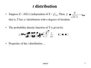
Is known? yes no Is the population normal? Is the population normal? yes no yes no Is n 30? Is n 30? Is n 30? yes no yes no yes no Give up Give up Remember This?
Is known? yes no Is the population normal? Is the population normal? yes no yes no Is n 30? Is n 30? Is n 30? yes no yes no yes no Give up Give up Remember This? The only case where the t distribution is needed
Table IV – t Percentiles • Table IV (p. 945) gives certain percentiles of t for certain degrees of freedom. • Open your book to page 945. • The columns give specific areas for upper-tails: • 0.40, 0.30, 0.20, 0.10, 0.05, 0.025, 0.01, 0.005. • The rows give specific degrees of freedom: • 1, 2, 3, …, 30, 40, 60, 120.
Table IV – t Percentiles • Look in the table at row 10, column 0.05: • The entry 1.812 means P(t > 1.812) = 0.05, when df = 10. • Draw a picture of the t distribution and this upper tail.
Table IV – t Percentiles • Since the t distribution is symmetric, we can also use the table for lower tails by making the t values negative. • So, what is P(t < –1.812), when df = 10? • Draw the picture.
Table IV – t Percentiles • The table allows us to look up certain percentiles, but it will not allow us to find probabilities (in general). • For example, what is P(t > 1.5) when df = 18? • We can’t tell exactly. • Look at row 18. You see 1.330 and 1.734, from columns 0.10 and 0.05, respectively. • Therefore, the best we can say is 0.05 < P(t > 1.5) < 0.10.
t-Table Practice • Find the following values of t : • 90th percentile when df = 25. • 10th percentile when df = 12. • 20th percentile when n = 5. • Find the following probabilities: • P(t > 2.518) when df = 21. • P(t < 0.851) when n = 41. • P(t > 2) when df = 8 (approx.).
t-Table Practice • Find the following values of t : • 90th percentile when df = 25. Answer: 1.316. • 10th percentile when df = 12. • 20th percentile when n = 5. • Find the following probabilities: • P(t > 2.518) when df = 21. • P(t < 0.851) when n = 41. • P(t > 2) when df = 8 (approx.).
t-Table Practice • Find the following values of t : • 90th percentile when df = 25. Answer: 1.316. • 10th percentile when df = 12. Answer: -1.356. • 20th percentile when n = 5. • Find the following probabilities: • P(t > 2.518) when df = 21. • P(t < 0.851) when n = 41. • P(t > 2) when df = 8 (approx.).
t-Table Practice • Find the following values of t : • 90th percentile when df = 25. Answer: 1.316. • 10th percentile when df = 12. Answer: -1.356. • 20th percentile when n = 5. Answer: -0.941. (df = 4) • Find the following probabilities: • P(t > 2.518) when df = 21. • P(t < 0.851) when n = 41. • P(t > 2) when df = 8 (approx.).
t-Table Practice • Find the following values of t : • 90th percentile when df = 25. Answer: 1.316. • 10th percentile when df = 12. Answer: -1.356. • 20th percentile when n = 5. Answer: -0.941. (df = 4) • Find the following probabilities: • P(t > 2.518) when df = 21. Answer: 0.01. • P(t < 0.851) when n = 41. • P(t > 2) when df = 8 (approx.).
t-Table Practice • Find the following values of t : • 90th percentile when df = 25. Answer: 1.316. • 10th percentile when df = 12. Answer: -1.356. • 20th percentile when n = 5. Answer: -0.941. (df = 4) • Find the following probabilities: • P(t > 2.518) when df = 21. Answer: 0.01. • P(t < 0.851) when n = 41. Answer: 0.80. (df = 40) • P(t > 2) when df = 8 (approx.).
t-Table Practice • Find the following values of t : • 90th percentile when df = 25. Answer: 1.316. • 10th percentile when df = 12. Answer: -1.356. • 20th percentile when n = 5. Answer: -0.941. (df = 4) • Find the following probabilities: • P(t > 2.518) when df = 21. Answer: 0.01. • P(t < 0.851) when n = 41. Answer: 0.80. (df = 40) • P(t > 2) when df = 8 (approx.). A:0.025 < P < 0.05.
TI-83 – Student’s t Distribution • However, the TI-83 will find probabilities for the t distribution (but it will not find percentiles!). • Press DISTR. • Select tcdf and press ENTER. • tcdf( appears in the display. • Enter the lower endpoint. • Enter the upper endpoint. • Enter the number of degrees of freedom (n – 1). • Press ENTER.
Example • Enter tcdf(1.812, E99, 10).
Example • Enter tcdf(1.812, E99, 10). • Scott, what did you get?
Example • Enter tcdf(1.812, E99, 10). • Scott, what did you get? • Ben, use the TI-83 to find P(t > 2) when df = 8.
Example • Enter tcdf(1.812, E99, 10). • Scott, what did you get? • Ben, use the TI-83 to find P(t > 2) when df = 8. • Nathan, is the answer between 0.025 and 0.05 (as we estimated earlier)?
Remember that! Hypothesis Testing with t • We should use the t distribution if • The population is normal (or nearly normal), and • is unknown, so we use s in its place, and • The sample size is small (n < 30). • Otherwise, we should not use t. • Either use Z or “give up.” • See the decision tree.
Hypothesis Testing with t • The hypothesis testing procedure is the same except for two steps. • Step 3: Find the value of the test statistic. • The test statistic is now • Step 4: Find the p-value. • We must look it up (estimate) in the t table, or use tcdf on the TI-83.
Example • Re-do Example 10.1 (by hand) under the assumption that is unknown.
Example • Re-do Example 10.1 (by hand) under the assumption that is unknown. • Mike D., what is step 1?
Example • Re-do Example 10.1 (by hand) under the assumption that is unknown. • Mike D., what is step 1? • Winchester, what is step 2?
Example • Re-do Example 10.1 (by hand) under the assumption that is unknown. • Mike D., what is step 1? • Winchester, what is step 2? • Everybody, do step 3.
Example • Re-do Example 10.1 (by hand) under the assumption that is unknown. • Mike D., what is step 1? • Winchester, what is step 2? • Everybody, do step 3. • Patrick, what did you get?
Example • Re-do Example 10.1 (by hand) under the assumption that is unknown. • Mike D., what is step 1? • Winchester, what is step 2? • Everybody, do step 3. • Patrick, what did you get? • Everybody, do step 4.
Example • Re-do Example 10.1 (by hand) under the assumption that is unknown. • Mike D., what is step 1? • Winchester, what is step 2? • Everybody, do step 3. • Patrick, what did you get? • Everybody, do step 4. • Nick, using the TI-83, what did you get?
Example • Glen, using the tables, what did you get?
Example • Glen, using the tables, what did you get? • Mladen, what is the decision?
Example • Glen, using the tables, what did you get? • Mladen, what is the decision? • Matt, what is the conclusion?
TI-83 – Hypothesis Testing When is Unknown • The TI-83 will perform a t-test. • Everybody, perform the following steps as we work Example 10.1 on the TI-83. • Press STAT. • Select TESTS. • Select T-Test. • A window appears requesting information. • Choose Stats.
TI-83 – Hypothesis Testing When is Unknown • Enter 0. • Enterx. • Enter s. (Remember, is unknown.) • Enter n. • Select the correct alternative hypothesis and press ENTER. • Select Calculate and press ENTER.
TI-83 – Hypothesis Testing When is Unknown • A window appears with the following information. • The title “T-Test” • The alternative hypothesis. • The value of the test statistic t. • The p-value. • The sample mean. • The sample standard deviation. • The sample size.
TI-83 – Hypothesis Testing When is Unknown • Josh, what does the TI-83 report as the value of t ? • Michael K., what does the TI-83 report as the p-value?
Let’s Do It! • Let’s do it! 10.3, p. 582 – Study Time. • Check: • Is known? • Is the population normal? • What about the sample size? • Let’s do it! 10.4, p. 583 – pH Levels.