Download
1 / 22
220 likes | 354 Views
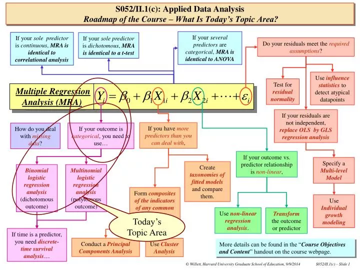
If your several predictors are categorical , MRA is identical to ANOVA. If your sole predictor is continuous , MRA is identical to correlational analysis. If your sole predictor is dichotomous , MRA is identical to a t-test. Do your residuals meet the required assumptions ?.

E N D
If your several predictors are categorical, MRA is identical to ANOVA If your sole predictor is continuous, MRA is identical to correlational analysis If your solepredictor is dichotomous, MRA is identical to a t-test Do your residuals meet the required assumptions? Use influence statistics to detect atypical datapoints Test for residual normality Multiple Regression Analysis (MRA) If your residuals are not independent, replace OLS byGLS regression analysis If you have more predictors than you can deal with, If your outcome is categorical, you need to use… How do you deal with missing data? If your outcome vs. predictor relationship isnon-linear, Specify a Multi-level Model Create taxonomies of fitted models and compare them. Binomiallogistic regression analysis (dichotomous outcome) Multinomial logistic regression analysis (polytomous outcome) Form composites of the indicators of any common construct. Use Individual growth modeling Use non-linear regression analysis. Transform the outcome or predictor Today’s Topic Area If time is a predictor, you need discrete-time survival analysis… Conduct a Principal Components Analysis Use Cluster Analysis More details can be found in the “Course Objectives and Content” handout on the course webpage. S052/II.1(c): Applied Data AnalysisRoadmap of the Course – What Is Today’s Topic Area?
Syllabus Sections II.1(c) & II.1(d),Fitting Taxonomies of Nested Logit Models, contain: • Fitting a taxonomy of logistic regression models (#3 - #5). • Some oddities in the PROC LOGISTIC output (#6 - #9). • Picking a final model and conducting a GLH test of model parameters using differencesin the –2LL statistic (#10 - #11). • Anti-logging parameter estimates to form fitted odds-ratios when an interaction is present (#12 - #16). • Fitting logistic trend lines for prototypical individuals (#17 - #18). • Appendix I: What is this AIC statistic, that accompanies the -2LL statistic everywhere it goes (#19-#22)? S052/II.1(c): Fitting Taxonomies of Logistic Regression (“Logit”) Models Printed Syllabus – What Is Today’s Topic? Please check inter-connections among the Roadmap, the Daily Topic Area, the Printed Syllabus, and the content of today’s class when you pre-read the day’s materials.
Our research question, asks: Do married Canadian women have a higher probability of being at-home mothers (versus joining the workforce) when they have children at home and their husbands earn higher salaries? (in 1977, at least!) Notice I added predictor CHILD into the mix. S052/II.1(c): Fitting Taxonomies of Logistic Regression (“Logit”) Models Basic Details of the AT_HOME dataset 1 15 1 1 13 1 1 45 1 1 23 1 1 19 1 1 7 1 1 15 1 0 7 1 1 15 1 1 23 1 1 23 1 0 13 1 1 9 1 …
You can include the main effects of, and interactions among, several predictors. They are simply inserted into the denominator on the RHS of the logistic model, in the exponent … I have fitted this short hypothesized taxonomy of logistic regression models using PROC LOGISTIC, in PC-SAS, as usual … in Data-Analytic Handout II.1(c).1 S052/II.1(c): Fitting Taxonomies of Logistic Regression (“Logit”) Models Specifying A Taxonomy of Hypothesized Logistic Regression Models Multiple predictors can easily be included in the logistic regression model …
Standard data input, and variable naming Standard creation of a two-way interaction between HUBSAL and CHILD Notice that, in PROC LOGISTIC, you can only specify one model per PROC paragraph The taxonomy contains a straightforward “build up” of the main effects of, and interaction between, HUBSAL and CHILD. S052/II.1(c): Fitting Taxonomies of Logistic Regression (“Logit”) Models FittingA Taxonomy of Hypothesized Logit Models in PC-SAS PC-SAS code from Data-Analytic Handout II.1(c).1 … *-----------------------------------------------------------------------* Input the data, name and label the variables in the dataset *-----------------------------------------------------------------------*; * Input the data from the external file; DATA AT_HOME; INFILE 'C:\DATA\S052\AT_HOME.txt'; INPUT HOME HUBSAL CHILD; LABEL HOME = 'Working as a Homemaker' HUBSAL = 'Husband''s annual salary ($1000)' CHILD = 'Children present in the home'; * Create a two-way interaction between HUBSAL and CHILD; HUBxCHLD = HUBSAL*CHILD; *-----------------------------------------------------------------------* Fitting a short taxonomy of interesting nested logistic regression models *-----------------------------------------------------------------------*; PROCLOGISTIC DATA=AT_HOME; MODEL HOME(event='1') = HUBSAL / MAXITER=50 RSQUARE; PROCLOGISTIC DATA=AT_HOME; MODEL HOME(event='1') = CHILD / MAXITER=50 RSQUARE; PROCLOGISTIC DATA=AT_HOME; MODEL HOME(event='1') = HUBSAL CHILD / MAXITER=50 RSQUARE; PROCLOGISTIC DATA=AT_HOME; MODEL HOME(event='1') = HUBSAL CHILD HUBxCHLD / MAXITER=50 RSQUARE;
Here’s an oddity of the output: • The -2LL statistic for the fitted model is listed under “Intercept & Covariates.” • Meaning that this is the fitted model that contains (the intercept and) any predictor(s), here HUBSAL • For this model, -2LL = 504.05. • Here’s another oddity: • You also get (without prompting) the -2LL statistic for the unconditional or “Null”model. • Meaning that this is a model that contains only an intercept. • For this model, -2LL = 526.45 . According to the approximate Wald Tests, the HUBSAL slope is not zero, in the population. On average, the fitted odds that a woman will remain at home are 1.084 times odds for a woman whose husband earns $1000 less S052/II.1(c): Fitting Taxonomies of Logistic Regression (“Logit”) Models Output From The Fitted Taxonomy Output from the first model in the taxonomy … Model Fit Statistics Intercept Intercept and Criterion Only Covariates AIC 528.449 508.050 -2 Log L 526.449 504.050 Analysis of Maximum Likelihood Estimates Standard Wald Parameter DF Estimate Error Chi-Square Pr > ChiSq Exp(Est) Intercept 1 -0.2372 0.2627 0.8151 0.3666 0.789 HUBSAL 1 0.0808 0.0184 19.2676 <.0001 1.084 Odds Ratio Estimates Point 95% Wald Effect Estimate Confidence Limits HUBSAL 1.084 1.046 1.124
Here’s the -2LL statistic for the model that we’ve fitted, containing an intercept and the main effect of CHILD Notice that the value of the -2LL statistic for the Null Model, remains the same throughout the entire taxonomy. Each parameter is non-zero in the population, even by the approximate Wald tests On average, the fitted odds that a woman with children will remain at home are 11.824 times odds for a woman without children. S052/II.1(c): Fitting Taxonomies of Logistic Regression (“Logit”) Models Output From The Fitted Taxonomy Output from the second model in the taxonomy … Model Fit Statistics Intercept Intercept and Criterion Only Covariates AIC 528.449 415.626 -2 Log L 526.449 411.626 Analysis of Maximum Likelihood Estimates Standard Wald Parameter DF Estimate Error Chi-Square Pr > ChiSq Exp(Est) Intercept 1 -0.6061 0.1794 11.4107 0.0007 0.545 CHILD 1 2.4701 0.2471 99.9078 <.0001 11.824 Odds Ratio Estimates Point 95% Wald Effect Estimate Confidence Limits CHILD 11.824 7.285 19.192
Value of the -2LL statistic for the model that we’ve fitted, containing an intercept & the main effects of HUBSAL and CHILD All parameters are non-zero in the population, by the approximate Wald tests We could interpret these as estimated odds-ratios, too … but let’s wait because we are about to discover that the two-way interaction of HUBSAL and CHILD has a statistically significant relationship with outcome AT_HOME!!! S052/II.1(c): Fitting Taxonomies of Logistic Regression (“Logit”) ModelsOutput From The Fitted Taxonomy Output from the third model in the taxonomy … Model Fit Statistics Intercept Intercept and Criterion Only Covariates AIC 528.449 394.086 -2 Log L 526.449 388.086 Analysis of Maximum Likelihood Estimates Standard Wald Parameter DF Estimate Error Chi-Square Pr > ChiSq Exp(Est) Intercept 1 -1.9479 0.3536 30.3448 <.0001 0.143 HUBSAL 1 0.0922 0.0203 20.6017 <.0001 1.097 CHILD 1 2.5821 0.2613 97.6468 <.0001 13.224 Odds Ratio Estimates Point 95% Wald Effect Estimate Confidence Limits HUBSAL 1.097 1.054 1.141 CHILD 13.224 7.924 22.070
-2LL statistic for the model that we’ve fitted, containing an intercept, the main effects of HUBSAL & CHILD, and their interaction Everything is non-zero in the population, even by the approximate Wald tests For the same reason that you must be careful interpreting main effects in models that contain interactions, I suggest that you do not even try to interpret these exponentiated estimates when there is an interaction present in the model!!! Instead, use the approach that I document later in the presentation ... S052/II.1(c): Fitting Taxonomies of Logistic Regression (“Logit”) Models Output From The Fitted Taxonomy Output from the fourth model in the taxonomy … Model Fit Statistics Intercept Intercept and Criterion Only Covariates AIC 528.449 391.971 -2 Log L 526.449 383.971 Analysis of Maximum Likelihood Estimates Standard Wald Parameter DF Estimate Error Chi-Square Pr > ChiSq Exp(Est) Intercept 1 -1.4613 0.4091 12.7600 0.0004 0.232 HUBSAL 1 0.0591 0.0249 5.6476 0.0175 1.061 CHILD 1 1.5037 0.5826 6.6618 0.0099 4.498 HUBxCHLD 1 0.0838 0.0417 4.0305 0.0447 1.087 Odds Ratio Estimates Point 95% Wald Effect Estimate Confidence Limits HUBSAL 1.061 1.010 1.114 CHILD 4.498 1.436 14.092 HUBxCHLD 1.087 1.002 1.180
Main effects of both CHILD and HUBSAL are consistently preserved, even when the other is present. The two-way interaction of HUBSAL and CHILD has a statistically significant effect on the outcome. –2LL statistic declines interpretably from its value in the null model as specific predictors are added across the taxonomy. Notice that I’ve used the approximate Wald tests to provide the approximate p-values for the table S052/II.1(c): Fitting Taxonomies of Logistic Regression (“Logit”) Models Taxonomy Of Fitted Logistic Regression Models Here’s the complete taxonomy of fitted models … Table II.1(c).1. Taxonomy of nested logistic regression models that display the fitted relationship between whether a married woman works in the home, as a homemaker (versus joining the labor force) as a function of her husband’s salary and the presence of children in their home, for a national sample of 434 married Canadian women in 1976. Key: ~ p<.10; * p<.05; ** p<.01; *** p<.001
Single-parameter Wald tests are only approximate, but still a useful guide for taxonomy building. However, methodologists recommend that you use the GLH approach to test the impact of any important predictor, or any important group of predictors. • For instance, to test the impact of the interaction: • H0: HUBSALxCHLD = 0, controlling for the main effects of HUBSAL and CHILD • Identify full and reduced fitted models, as usual. • Obtain the difference in their –2LL goodness-of-fit statistics. • Compare it to a critical value from a 2 distribution with df equal to the number of constraints imposed in the test, at a chosen α-level. Full Model (M4), -2LL statistic = 383.97 Reduced Model (M3), -2LL statistic = 388.09 Difference in -2LL statistic = 4.12 Critical value, 2 (1 df, α=.05) = 3.84 Decision: Reject H0 We conclude that the effect of the husband’s salary on the woman’s decision to remain in the home depends on the presence of children S052/II.1(c): Fitting Taxonomies of Logistic Regression (“Logit”) Models Conducting a GLH Test By Comparing Full & Reduced Fitted Logistic Regression Models Table II.1(c).1. Taxonomy of nested logistic regression models that display the fitted relationship between whether a married woman works in the home, as a homemaker (versus joining the labor force) as a function of her husband’s salary and the presence of children in their home, for a national sample of 434 married Canadian women in 1976. Preferred “final” model? Key: ~p<.10; *p<.05; **p<.01; ***p<.001
Still use theantilog/odds-ratio method to interpret parameter estimates directly but, because a two-way interaction is present, you cannot interpret the main effects separately from the effect of the interaction. Why? Because the presence of an interaction means that one predictor’s effect differs by levels of the other … so, there are two possible ways of viewing of the results. S052/II.1(d): Logistic Regression (“Logit”) Analysis/Interpreting the Fitted Model Interpreting the Final Fitted Model Using Fitted Odds-Ratios Now that we know that Model M4 is the final fitted logistic model, let’s interpret its estimated parameters … View #1 You can interpret the effect of HUBSAL at different levels of CHILD View #2 You can interpret the effect of CHILD at different levels of HUBSAL
Notice how the presence of the interaction has lead the impact of HUBSAL to differ by levels of CHILD S052/II.1(d): Logistic Regression (“Logit”) Analysis/Interpreting the Fitted Model Antilogging Parameter Estimates to Interpret Using Odds-Ratios View #1: Here are the fitted relationships between HOME & HUBSALat different levels of CHILD … When CHILD=0, the fitted relationship between HOME and HUBSAL is: When CHILD=1, the fitted relationship between HOME and HUBSAL is:
When CHILD=0, the fitted relationship between HOME and HUBSAL is: On average, in the population,when there areno children in the home, the fitted odds that a woman will remain in home are 1.061times the fitted odds when the husband’s salary is $1000 lower. When CHILD=1, the fitted relationship between HOME and HUBSAL is: On average, in the population, when there are children in the home, the fitted odds that a woman will remain in home are 1.154 times the fitted odds when the husband’s salary is $1000 lower. S052/II.1(d): Logistic Regression (“Logit”) Analysis/Interpreting the Fitted Model Antilogging Parameter Estimates to Interpret Using Odds-Ratios
When HUBSAL=$10,000,the fitted relationship between HOME and CHILD is: Notice how the presence of the interaction has lead the impact of CHILD to differ by levels of HUBSAL When HUBSAL=$30,000, the fitted relationship between HOME and HUBSAL is: S052/II.1(d): Logistic Regression (“Logit”) Analysis/Interpreting the Fitted ModelAntilogging Parameter Estimates to Interpret Using Odds-Ratios View #2: Here are the fitted relationships between HOME & CHILD at different levels of HUBSAL …
On average, in the population, when a husband earns $10,000, the fitted odds that a woman with children will remain in the home are 10.42 times the fitted odds that a woman without children will do the same. On average, in the population, when a husband earns $30,000, the fitted odds that a woman with children will remain in the home are 55.92 times the fitted odds that a woman without children will do the same. S052/II.1(d): Logistic Regression (“Logit”) Analysis/Interpreting the Fitted ModelAntilogging Parameter Estimates to Interpret Using Odds-Ratios When HUBSAL=$10,000 the fitted relationship between HOME and CHILD is: When HUBSAL=$30,000, the fitted relationship between HOME and HUBSAL is:
HUBSAL ranges from 1 through 45, in families that have children in the home. Plot fitted HOME/HUBSAL relationship over these ranges of HUBSALin families with, and without, children!! Already figured out requisite fitted models on Slide #13 HUBSAL ranges from 1 through 35, in families that have no children in the home. S052/II.1(d): Logistic Regression (“Logit”) Analysis/Interpreting the Fitted Model Obtaining The Statistics Necessary For Creating Reasonable Fitted Plots Finally, you can also use the standardmethod of plotting fitted trend lines for prototypical folk to interpret the magnitudes and directions of the effects present in the final model … Sample median, 1st percentile & 99th percentile of husband’s salary (in $1000), by presence of children in the home, for 434 married Canadian women in 1976 (from Data-Analytic Handout II.1(d).1). „ƒƒƒƒƒƒƒƒƒƒƒƒƒƒƒƒƒƒƒ…ƒƒƒƒƒƒƒƒƒƒƒƒ…ƒƒƒƒƒƒƒƒƒƒƒƒ…ƒƒƒƒƒƒƒƒƒƒƒƒ† ‚ ‚ P1 ‚ Median ‚ P99 ‚ ‡ƒƒƒƒƒƒƒƒƒ…ƒƒƒƒƒƒƒƒƒˆƒƒƒƒƒƒƒƒƒƒƒƒˆƒƒƒƒƒƒƒƒƒƒƒƒˆƒƒƒƒƒƒƒƒƒƒƒƒ‰ ‚Husband's‚Children ‚ ‚ ‚ ‚ ‚annual ‚present ‚ ‚ ‚ ‚ ‚salary ‚in the ‚ ‚ ‚ ‚ ‚($1000) ‚home ‚ ‚ ‚ ‚ ‚ ‡ƒƒƒƒƒƒƒƒƒ‰ ‚ ‚ ‚ ‚ ‚0 ‚ 1.00‚ 13.00‚ 35.00‚ ‚ ‡ƒƒƒƒƒƒƒƒƒˆƒƒƒƒƒƒƒƒƒƒƒƒˆƒƒƒƒƒƒƒƒƒƒƒƒˆƒƒƒƒƒƒƒƒƒƒƒƒ‰ ‚ ‚1 ‚ 1.00‚ 15.00‚ 45.00‚ Šƒƒƒƒƒƒƒƒƒ‹ƒƒƒƒƒƒƒƒƒ‹ƒƒƒƒƒƒƒƒƒƒƒƒ‹ƒƒƒƒƒƒƒƒƒƒƒƒ‹ƒƒƒƒƒƒƒƒƒƒƒƒŒ
The “View #2” odds-ratios estimated earlier, which compared the fitted odds that a woman with a child would remain home (vs. be at work), to the fitted odds for a woman who had no child, refer to comparisons of fitted probability at $10K and $30K, by child & no-child. Child Present No Child S052/II.1(d): Logistic Regression (“Logit”) Analysis/Interpreting the Fitted Model Fitted Plots For Prototypical Married Canadian Women, In 1976 • General Conclusions • On average, in the population: • 1. Husband’s Salary: Women whose husbands earn more have a higher probability of remaining at home than those whose husband’s earn less. • 2. Presence of Children in the Home: Regardless of the husband’s salary, women with children have a higher probability of being at home than women with no children. • Interaction: Effect of children differs by husband’s salary. The “View #1” odds-ratios estimated earlier, comparing the fitted odds that two women whose husband’s wages were $1K apart will remain at home (vs. be at work) when achild is present (1.154) and when a child is not present (1.061) represent the difference in slopes of these two fitted logistic curves.
AIC stands for Akaike Information Criterion and is printed out when the method of maximum likelihood (ML) estimation is used. In Model #4, here: AIC =391.971 • It’s always a little bigger than the –2LL statistic itself, because: • AIC = -2LL + 2(# of parameters in model) • It’s a badness-of-fit statistic like –2LL (and so, “smaller is better” or “bigger is worse”). • By being bigger, it’s supposed to “penalize” the –2LL statistic for being too optimistic when the model is “overloaded” with “unnecessary” predictors. S052/II.1(d): Fitting Taxonomies of Logistic Regression (“Logit”) Models Appendix 1: What’s The AIC Statistic, Cited Along With The –2LL Statistic? Model Fit Statistics Intercept Intercept and Criterion Only Covariates AIC 528.449 391.971 SC 532.522 408.263 -2 Log L 526.449 383.971 R-Square 0.2798 Max-rescaled R-Square 0.3982
Notice that the AIC statistic declines as the fit improves, just like the -2LL statistic does S052/II.1(d): Fitting Taxonomies of Logistic Regression (“Logit”) Models Appendix 1: What’s The AIC Statistic, Cited Along With The –2LL Statistic? Here’s the fitted taxonomy with the AIC statistic included… Table II.1(c).1. Taxonomy of nested logistic regression models that display the fitted relationship between whether a married woman works in the home, as a homemaker (versus joining the labor force) as a function of her husband’s salary and the presence of children in their home, for a national sample of 434 married Canadian women in 1976. Key: ~p<.10; *p<.05; **p<.01; ***p<.001
We say that model #4 is nested within model #5 because you can obtain model #4 from model #5 by directly constraining it. Because it “corrects for” the number of predictors in the model, some people say that AIC can be used to compare non-nested models(provided they have been fitted to the same data). When two models are nestedyou can compare their fits using differences in the –2LL statistic, as we have done. But, the AIC statistic of Model #2 is less than the AIC statistic for Model #1, supposedly confirming that Model #2 fits better than Model #1 Models #1 and #2 are not nested. S052/II.1(d): Fitting Taxonomies of Logistic Regression (“Logit”) Models Appendix 1: What’s The AIC Statistic, Cited Along With The –2LL Statistic? Comparing fitted models using the –2LL and AIC statistics … Table II.1(c).1. Taxonomy of nested logistic regression models that display the fitted relationship between whether a married woman works in the home, as a homemaker (versus joining the labor force) as a function of her husband’s salary and the presence of children in their home, for a national sample of 434 married Canadian women in 1976. Key: ~p<.10; *p<.05; **p<.01; ***p<.001
Gelman & Rubin (1995) comment that the AIC statistic (and others like it, including BIC, SC, etc.) are “off-target and only by serendipity manage to hit the target in special circumstances” I agree with Gelman & Rubin … “use [AIC] with care, and only when more rigorous traditional methods are not applicable.” S052/II.1(d): Fitting Taxonomies of Logistic Regression (“Logit”) Models Appendix 1: What’s The AIC Statistic, Cited Along With The –2LL Statistic? How should you judge differences in the magnitude of AIC between models? … very cautiously indeed!!! Raftery (1995) suggests that a difference in AIC of: 0-2 is “weak” evidence of a difference in fit, 2-6 is “positive” 6-10 is “strong” >10 is “very strong