Download
1 / 29
420 likes | 747 Views
From Unit Root To Cointegration. Putting Economics into Econometrics. Nelson and Plosser (1982) - Most macroeconomic Variables Are non Stationary. Economics - Many variables have stable relationships. Consumption - Income Prices - Wages Prices at Home - Prices Abroad.

E N D
From Unit Root To Cointegration Putting Economics into Econometrics
Nelson and Plosser (1982) - Most macroeconomic Variables Are non Stationary • Economics - Many variables have stable relationships. • Consumption - Income • Prices - Wages • Prices at Home - Prices Abroad Can we use the Unit Root Technology to distinguish between variables which are not correlated and variables which are?
Economic theory tells us that between them there should be (at least in the long run) a relation like Let’s try to do a regression between these variables Modelling Consumption by OLS Variable Coefficient Std.Error t-value t-prob PartR^2 Constant 10.420 0.87726 11.877 0.0000 0.5876 Income 0.79680 0.0070914 112.361 0.0000 0.9922 R^2 = 0.992219 F(1,99) = 12625 [0.0000] \sigma = 0.834499 DW = 2.05 RSS = 68.94243871 for 2 variables and 101 observations The Regression is not Spurious - Although the Two Variables are Not Stationary. This is a Long Run Relationship
COINTEGRATION If exist a relation between non stationary series, like Such that the residuals of the regression are stationary, then the variables in question are said to be Cointegrated There is a Long Run Relationship towards which they always come back
Consider The Following Two Series - Income and Consumption They are clearly not stationary But they seem to move together
Let’s try again to regression between consumption and Income (this time with real data!) Modelling CONS by OLS The present sample is: 1954 (2) to 1992 (3) Variable Coefficient Std.Error t-value t-prob PartR^2 Constant -183.97 30.704 -5.992 0.0000 0.1911 INC 1.1886 0.034442 34.511 0.0000 0.8868 R^2 = 0.886822 F(1,152) = 1191 [0.0000] DW = 0.360 RSS = 3208.248561 for 2 variables and 154 observations Now the results are not so good! But Economic Theory tells us that a relation exist - How can we distinguish between the regression above and a spurious regression? - We Need a Formal Test
First Test: Cointegrating Regression Durbin Watson Test (CRDW) If the residual are non stationary, DW will go to 0 as the sample size increases. So “large” values of DW are taken as evidence for rejection of the null hypothesis of NO COINTEGRATION In the previous example you have only weak cointegration (Can you tell if there is some theoretical reason for that?) Modelling CONS by OLS The present sample is: 1954 (2) to 1992 (3) Variable Coefficient Std.Error t-value t-prob PartR^2 Constant -183.97 30.704 -5.992 0.0000 0.1911 INC 1.1886 0.034442 34.511 0.0000 0.8868 R^2 = 0.886822 F(1,152) = 1191 [0.0000] DW = 0.360
Second Test: Cointegrating Regression ADF test (CRADF) 1 - Perform the cointegrating regression 2 - ADF teat on the residual see the table at page 233 for the critical values of both tests
First Step Engle-Granger: ADF Test on the residuals (ECM) EQ(19) Modelling DECM by OLS (using Data.in7) The present sample is: 1953 (4) to 1992 (3) Variable Coefficient Std.Error t-value t-prob PartR^2 Constant -0.013457 0.21074 -0.064 0.9492 0.0000 ECM_1 -0.18144 0.046341 -3.915 0.0001 0.0905 R^2 = 0.0905328 F(1,154) = 15.33 [0.0001] \sigma = 2.63218 DW = 1.93 RSS = 1066.973229 for 2 variables and 156 observations
Second Test: Cointegrating Regression ADF test (CRADF) 1 - Perform the cointegrating regression 2 - ADF test on the residual see the table on page 233 for the critical values of both tests
Second Step - The residuals of the cointegration regression are entered in a more general dynamic specification of the relation between Y and X like: Another test for cointegration If we cannot reject the null, there is no error correction mechanism operating and so the variables do not cointegrate
Applications Of Engle-Granger Two-Step Procedure Cointegration in Practice
Testing For Cointegration • Pretest the variables for their order of integration • Estimate the Long Run Equilibrium Relationship • Estimate the Error Correction Model • Assess Model Adequacy
Pretest the variables for their order of integration • By definition cointegration necessitates that the variables be • integrated of the same order • Use DF or ADF tests to determine the order of integration • If variables are I(0) - Standard Time Series Methods • If the variables are integrated of different order • (one I(0), one I(1) or I(2) etc) than it is possible to conclude • that the two variables are not cointegrated • If the variables are I(1), or are integrated of the same order, • go on
Estimate the Long Run Equilibrium Relationship Estimate the long run relationship If the variables are cointegrated, an OLS regression yields a “super-consistent” estimator of the cointegrated parameter 0 and 1. There is a strong linear relationship. Use the residual (e) of the estimated long run relationship. If (e) is STATIONARY (according to DF criteria) than we can conclude that the series are COINTEGRATED
Estimate the Error Correction Model If the variables are cointegrated, the residual from the equilibrium regression can be used to estimate the Error Correction Model Using the saved residual from the estimation of the long-run relationship, we can estimate the ECM as: Granger’s representation theorem: if a set of variables are cointegrated then there always exists an error correcting formulation of the dynamic model and vice versa
Assess Model Adequacy Asses if the ECM model you have estimate is appropriate using a General - Specific modelling approach
Some authors are uncomfortable with the two stage approach. Any mistake introduced in the first step, is carried forward in the second step. As long as the equation is balanced, an unrestricted ECM model can be at least as efficient as a two step EG method in defining long run relationships and short run dynamics This means estimating the following ECM model
Consider for example the Consumption-Income model analysed in a previous lecture. Modelling LC by OLS Variable Coefficient Std.Error t-value t-prob PartR^2 Constant 0.013285 0.080615 0.165 0.8696 0.0004 LYd 0.98530 0.011002 89.557 0.0000 0.9925 DW = 0.322 First step: Second Step:
Same Estimation with Free Parameters Does it make a difference?
In this case not very much From the long term relation estimation: Inserting this term in the dynamic equation we have estimated: Substituting the first in the second we have
Therefore with EG two step we obtain With the standard ECM procedure we have: Sometimes the second way is more efficient
Second Problem We have assumed that Economic Theory can guide in determining the dependent and the independent variable, like in the Consumption Function. What if this is not possible?
Given three variables (y,w,z) you have three possible long run relationship, and three possible ECM models
These weaknesses limit the applicability of the EG two step procedure. We need to introduce a technique that considers cointegration not only between pairs of variables, but also in a system This technique is the ML approach of Johansen