Download
1 / 40
400 likes | 571 Views
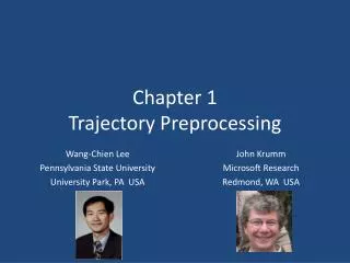
Chapter 1 Trajectory Preprocessing. Wang- Chien Lee Pennsylvania State University University Park, PA USA. John Krumm Microsoft Research Redmond, WA USA. Mobile Commerce. Local weather. Navigation. Location-Based Services. Traffic info. Logistics. Geographical Information

E N D
Chapter 1Trajectory Preprocessing Wang-Chien Lee Pennsylvania State University University Park, PA USA John Krumm Microsoft Research Redmond, WA USA
Mobile Commerce Local weather Navigation Location-Based Services Traffic info Logistics Geographical Information System (GIS) Emergency service Tracking
System Model for LBSs • The locations of tracked moving objects are reported to the location server via wireless communications. • The LBS applications submit queries to the server to retrieve moving object data for analysis or other application needs.
Trajectories {< x1, y1, t1>, < x2, y2, t2>, ..., < xN, yN, tN>} • Positioning technologies • Global positioning system (GPS) • Network-based (e.g., using cellular or wifi access points) • Dead-Reckoning (for estimation)
Trajectory Preprocessing • Problems to solve with trajectories • Lots of trajectories → lots of data • Noise complicates analysis and inference • Employ the data reduction and filtering techniques • Specialized data compression for trajectories • Principled filtering techniques
Performance Metrics • Trajectory data reduction techniques aims to reduce trajectory size w/o compromising much precision. • Performance Metrics • Processing time • Compression Rate • Error Measure • The distance between a location on the original trajectory and the corresponding estimated location on the approximated trajectory is used to measure the error introduced by data reduction. • Examples are Perpendicular Euclidean Distance or Time Synchronized Euclidean Distance.
Illustration of Error Measures • Perpendicular Euclidean Distance • Time Synchronized Euclidean Distance
Trajectory Data Reduction • Classification of Data Reduction Techniques. • Batched Compression: • Collect full set of location points and then compress the data set for transmission to the location server. • Applications: content sharing sites such as Everytrail and Bikely. • Techniques include Douglas-Peucker Algorithm, top-down time-ratio (TD-TR), and Bellman's algorithm. • On-line Data Reduction • Selective on-line updates of the locations based on specified precision requirements. • Applications: traffic monitoring and fleet management. • Techniques include Reservoir Sampling, Sliding Window, and Open Window.
Batch Compression - Douglas-Peucker (DP) Algorithm • Preserve directional trends in the approximated trajectory using the perpendicular Euclidean distance as the error measure. • Replace the original trajectory by an approximate line segment. • If the replacement does not meet the specified error requirement, it recursively partitions the original problem into two subproblems by selecting the location point contributing the most errors as the split point. • This process continues until the error between the approximated trajectory and the original trajectory is below the specified error threshold.
Illustration of DP Algorithm • Split at the point with most error. • Repeat until all the errors < given threshold
Batch Compression - Top-Down Time-Ratio (TDTR) and Bellman Algorithms • DP uses perpendicular Euclidean distance as the error measure. Also, it’s heuristic based, i.e., no guarantee that the selected split points are the best choice. • TDTR uses time synchronized Euclidean distance as the error measure to take into account the geometric and temporal properties of object movements. • Bellman Algorithm employs dynamic programming technique to ensure that the approximated trajectory is optimal • Its computational cost is high.
Joke The one about the guy who joins a monastery
On-line Compression –Sliding Window • Fit the location points in a growing sliding window with a valid line segment and continue to grow the sliding window until the approximation error exceeds some error bound. • First initialize the first location point of a trajectory as the anchor point pa and then starts to grow the sliding window • When a new location point pi is added to the sliding window, the line segment pa pi is used to fit all the location points within the sliding window. • As long as the distance errors against the line segment pa pi are smaller than the user-specified error threshold, the sliding window continues to grow. Otherwise, the line segment pa pi-1 is included as part of the approximated trajectory and pi is set as the new anchor point. • The algorithm continues until all the location points in the original trajectory are visited.
Sliding Window - Illustration • While the sliding window grows from {p0} to {p0, p1, p2, p3}, all the errors between fitting line segments and the original trajectory are not greater than the specified error threshold. • When p4 is included, the error for p2 exceeds the threshold, so p0p3 is included in the approximate trajectory and p3 is set as the anchor to continue.
Open Window • Different from the sliding window, choose location points with the highest error in the sliding window as the closing point of the approximating line segment as well as the new anchor point. • When p4 is included, the error for p2 exceeds the threshold, so p0p2 is included in the approximate trajectory and p2 is set as the anchor to continue.
Part 1 Summary Trajectory Data Compression • Batch • Douglas-Peucker (DP) • Top-Down Time Ratio (TDTR) – time included • Bellman – dynamic programming • On-line • Sliding window • Open window (variation of sliding window)
Part 2 - Filtering • Goals • Smooth noise & outliers • Infer higher level values (e.g. speed) • Techniques • Mean and median • Kalman filter • Particle filter
Running Example • Track a moving person in (x,y) • 1075 (x,y) measurements • Δ = 1 second • Manually added outliers Notation measurement vector actual location noise zero mean standard deviation = ~4 meters
Mean Filter • Also called “moving average” and “box car filter” • Apply to x and y measurements separately Filtered version of this point is mean of points in solid box zx t • “Causal” filter because it doesn’t look into future • Causes lag when values change sharply • Help fix with decaying weights, e.g. • Sensitive to outliers, i.e. one really bad point can cause mean to take on any value • Simple and effective (I will not vote to reject your paper if you use this technique)
Mean Filter outlier 10 points in each mean • Outlier has noticeable impact • If only there were some convenient way to fix this …
Median Filter Filtered version of this point is mean median of points in solid box Insensitive to value of, e.g., this point zx t Median is way less sensitive to outliners than mean median (1, 3, 4, 7, 1 x 10¹⁰) = 4 mean (1, 3, 4, 7, 1 x 10¹⁰) ≈ 2 x 10⁹
Median Filter outlier 10 points in each median Outlier has noticeable less impact
Joke The one about the statisticians who go hunting
Kalman Filter Assumed trajectory is parabolic • Mean and median filters assume smoothness • Kalman filter adds assumption about trajectory My favorite book on Kalman filtering Big difference #1: Kalman filter includes (helpful) assumptions about behavior of measured process Weight data against assumptions about system’s dynamics dynamics data
Kalman Filter Kalman filter separates measured variables from state variables Running example: measure (x,y) coordinates (noisy) Measure: Running example: estimate location and velocity (!) Infer state: Big difference #2: Kalman filter can include state variables that are not measured directly
Kalman Filter Measurements Measurement vector is related to state vector by a matrix multiplication plus noise. Running example: • In this case, measurements are just noisy copies of actual location • Makes sensor noise explicit, e.g. GPS has σ of around 4 meters
Kalman Filter Dynamics Insert a bias for how we think system will change through time location is standard straight-line motion velocity changes randomly (because we don’t have any idea what it actually does)
Kalman Filter Ingredients H matrix: gives measurements for given state Measurement noise: sensor noise φ matrix: gives time dynamics of state Process noise: uncertainty in dynamics model
Kalman Filter Recipe Big difference #3: Kalman filter gives uncertainty estimate in the form of a Gaussian covariance matrix • Just plug in measurements and go • Recursive filter – current time step uses state and error estimates from previous time step
Kalman Filter Velocity model: • Hard to pick process noise σs • Process noise models our uncertainty in system dynamics • Here it accounts for fact that motion is not a straight line “Tuning” σs (by trying a bunch of values) gives better result
Particle Filter Dieter Fox et al. WiFi tracking in a multi-floor building • Multiple “particles” as hypotheses • Particles move based on probabilistic motion model • Particles live or die based on how well they match sensor data
Particle Filter Dieter Fox et al. • Allows multi-modal uncertainty (Kalman is unimodal Gaussian) • Allows continuous and discrete state variables (e.g. 3rd floor) • Allows rich dynamic model (e.g. must follow floor plan) • Can be slow, especially if state vector dimension is too large(e.g. (x, y, identity, activity, next activity, emotional state, …) )
Particle Filter Ingredients • z = measurement, x = state, not necessarily same • Probability distribution of a measurement given actual value • Can be anything, not just Gaussian like Kalman • But we use Gaussian for running example, just like Kalman E.g. measured speed (in z) will be slower if emotional state (in x) is “tired” For running example, measurement is noisy version of actual value
Particle Filter Ingredients • Probabilistic dynamics, how state changes through time • Can be anything, e.g. • Tend to go slower up hills • Avoid left turns • Attracted to Scandinavian people • Closed form not necessary • Just need a dynamic simulation with a noise component • But we use Gaussian for running example, just like Kalman xi random vector xi-1
Particle Filter Algorithm Start with N instances of state vector xi(j) , i = 0, j = 1 … N i = i+1 Take new measurement zi Propagate particles forward in time with p(xi|xi-1), i.e. generate new, random hypotheses Compute importance weights wi(j) = p(zi|xi(j)), i.e. how well does measurement support hypothesis? Normalize importance weights so they sum to 1.0 Randomly pick new particles based on importance weights Goto 1 • Compute state estimate • Weighted mean (assumes unimodal) • Median
Particle Filter Dieter Fox et al. WiFi tracking in a multi-floor building • Multiple “particles” as hypotheses • Particles move based on probabilistic motion model • Particles live or die based on how well they match sensor data
Particle Filter Running Example Measurement model reflects true, simulated measurement noise. Same as Kalman in this case. Straight line motion with random velocity change. Same as Kalman in this case. location is standard straight-line motion velocity changes randomly (because we don’t have any idea what it actually does) Sometimes increasing the number of particles helps
Part 2 Summary • Measurement assumptions • Mean and median filters • Kalman filter • Particle filter