Download
1 / 24
240 likes | 378 Views
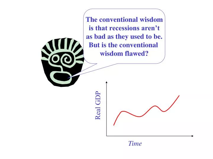
The conventional wisdom is that recessions aren’t as bad as they used to be. But is the conventional wisdom flawed?. Real GDP. Time. Romer's view.

E N D
The conventional wisdomis that recessions aren’t as bad as they used to be.But is the conventional wisdom flawed? Real GDP Time
Romer's view “The bottom line is . . . That [m]ajor macroeonomic indicators have not become dramatically more stable between the pre-World War I and Post World War I eras, and recessions have become only slightly less severe on average. Recessions have, however, become less frequent and more uniform over time.”1 1 Christina Romer.“Changes in Business Cycles: Evidence and Explanations,” Journal of Economic Perspectives, 13(2), Spring 1999, p. 23.
Romer's Method • Romer claims that the GDP series most frequently used for comparisons of pre-World War I with post-World War II cycles are excessively volatile because they were derived from data on the output of commodities (pig iron, coal, oil, wheat) . Most assumed that there was a one-to-one correspondence between output changes in these highly volatile industries and real GDP. Romer corrects for this defect and produces alternative estimates of real output.
Dates of Peaks and Troughs 1 1Post World War II dates are identical to NBER dates. Pre-WWII dates are computed using the methodology described by Romer(1999, p. 29). Source: Romer (1999)
Romers method of measuring business cycle severity Green shaded area is cumulative loss, given by the sum of the percentage shortfall for each month from April 1960 to may 1961 Index of Industrial Production P T 100 0 Apr 1960 Feb 1961 May 1961 Year/Month
Output Loss1 1Output loss is the sum of the percentage shortfall of industrial production in each month between the peak and he return to the peak. It is measured in percentage points. Source: Romer (1999)
Cycles differ in theirduration and severity (thoughduration is obviously oneaspect of the severity of a contraction). In examiningcycles in comparative perspective, are there any discerniblesimilarities or patterns?
Robert E. Lucas on Business Cycles “Though there is absolutely no theoretical reason to anticipate it, one is led by the facts to conclude that, with respect to the qualitative behavior of co-movements among series, business cycles are all alike.” (Lucas 1981, p. 218). Robert E. Lucas. “Understanding Business Cycles,” reprinted in Studies in Business-Cycle Theory by Robert E. Lucas. Cambridge, MA: MIT Press, 1981, 215-239.
“The regularities observed are in the co-movements among different [aggregate] time series, e.g. • Output movements across broadly defined sectors move together (they exhibit high conformity). • Production of producer and consumer durables exhibits much greater amplitude than production of nondurables. • Production and prices of agricultural goods and natural resources have lower than average conformity. • Business profits show high conformity and much greater amplitude than other series. • Prices are generally procyclical. • Short-term interest rates are procylical; long-term rates slightly so. • Monetary aggregates are procyclical.” (Lucas, 1981, p. 217).
Now we want to examine the behavior of keyaggregate-level timeseries in the 1979-83 periodin the U.S. Note that this periodspans two full contractions(recessions) and one full expansion.
Jan.80 is a peak; Jul. 80 is a trough; Jul. 81 is a peak; Dec. 1982 is a trough.
Now we want to examine the behavior of keyaggregate-level timeseries in the 1990-91 recession.