Download

1 / 72
750 likes | 956 Views
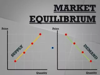
Market Equilibrium. S. Price. Pm. D. Qm. Quantity. Qs > QD Surplus Too many goods and services Producers cut price Qd increases Qs decreases Return to equilibrium. At a Price Above Equilibrium. S. Price. P1. Pm. D. Qm. Qd. Qs. Quantity.

E N D
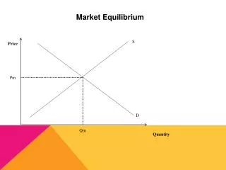
Market Equilibrium S Price Pm D Qm Quantity
Qs > QD • Surplus • Too many goods and services • Producers cut price • Qd increases • Qs decreases • Return to equilibrium At a Price Above Equilibrium S Price P1 Pm D Qm Qd Qs Quantity A surplus is where price is set above equilibrium causing QS>QD
Qd > Qs • Shortage • Not enough goods and services • Consumers bid up price • Qd decreases • Qs increases • Return to equilibrium At a Price Below Equilibrium S Price Pm P1 D Qm Qs Qd Quantity A shortage is where the price is set below equilibrium causing QD>QS
Conclusion • A market will tend toward equilibrium • If the price is not at equilibrium then market forces will work to move the market back toward equilibrium.
Consumer Surplus The difference between what consumers are willing to pay and the actual price paid for a commodity Definition: Measured by: The area below the demand curve and above the price line
Consumer Surplus S Price Consumer Surplus Pm D Qm Quantity
Producer Surplus Definition: Measured by: The difference between the revenue received by a producer and the the cost necessary to produce the good The area below the demand curve and above the price line
Producer Surplus S Price Producer Surplus Pm D Qm Quantity
Why is Equilibrium best? • Equilibrium represents the allocatively efficient point. • This is where Consumer Surplus and Producer Surplus are maximised • ie benefits to consumers and producers are at their greatest
Which is the allocatively efficient point? cars A 100 B 60 100 200 television
Which is the allocatively efficient point? cars Market for Cars A S price 100 B 60 D 100 100 quantity 200 television
Which is the allocatively efficent point? cars Market for Cars A S price 100 B 60 D 100 100 quantity 200 television
Net Welfare Benefit The combined values of the consumer and producer surpluses is referred to as the net welfare benefit. S Net welfare benefit. Pm D Qm
Allocative Efficiency and Market Equilibrium Markets allocate resources to the production of goods and services that satisfy consumers needs and wants. To be allocatively efficient a market must price and produce at equilibrium . Price Resources would be either over or under allocated to production and net welfare benefit would be reduced. S Any price other than $1.20 and any output level other than 400 units will result in a loss of allocative efficiency 1.80 1.50 1.20 0.90 0.60 0.30 To maintain allocative efficiency a market must be able to move freely to any new equilibrium D 200 400 600 800 Quantity
Any changes in the market where the forces of demand and supply are able to freely adjust to market conditions will still result in allocative efficiency.
A loss of Allocative Efficiency • A loss of allocative efficiency occurs when a market is not allowed to price and produce at equilibrium this will result from : • Price Controls(setting either a minimum or maximum price) • Imposition of a sales tax or subsidy • Imposition of a tariff or a quota (normally relates to internationally traded products) • All of these regulations set by the government will result in a dead weight loss and thus causing net social welfare to fall.
Deadweight Loss • When a market does not achieve equilibrium producer and consumer surplus will not be maximised • The loss in allocative efficiency is DWL • It is measured by the loss of CS and PS not offset by gains to other groups (eg government)
Deadweight Loss • Deadweight loss can be caused by: • Quotas • Price controls • Indirect Taxes • Subsidies
A Subsidy S Price Pm D Qm Quantity
A Subsidy Subsidies reduce costs and increase Supply S Price S+Subsidy Pm D Qm Quantity
A Subsidy Consumers pay the new equilibrium price - Pc S Price S+Subsidy Pm Pc D Qm Q’ Quantity
A Subsidy The per unit subsidy is represented by the vertical distance between the two supply curves S Price S+Subsidy Pm Pc D Qm Q’ Quantity
A Subsidy Producers receive higher price -Pp S Price Pp S+Subsidy Pm Pc D Qm Q’ Quantity
A Subsidy The total cost to the government is represented by the shaded area S Price Pp S+Subsidy Pm Pc D Qm Q’ Quantity
A Subsidy S Price Original CS Pp S+Subsidy Pm Pc D Qm Q’ Quantity
A Subsidy S Price New CS Pp S+Subsidy Pm The gain in CS represents the incidence of a subsidy on consumers Pc D Qm Q’ Quantity
A Subsidy S Price Old PS Pp S+Subsidy Pm Pc D Qm Q’ Quantity
A Subsidy S Price New PS Pp S+Subsidy Pm The gain in PS represents the incidence of a subsidy on producers Pc D Qm Q’ Quantity
A Subsidy S Price DWL Pp S+Subsidy Pm Pc D Qm Q’ Quantity
An Indirect Tax – Sales Tax S Price Pm D Qm Quantity
An Indirect Tax S+tax Indirect taxes increase costs and shift the supply curve to the left S Price Pm D Qm Quantity
An Indirect Tax S+tax Consumers pay the new equilibrium price - Pc S Price Pc Pm D Qm Quantity
An Indirect Tax S+tax The per unit tax is measured by the vertical distance between the two supply curves S Price Pc Pm D Q’ Qm Quantity
An Indirect Tax S+tax The producer recieves the lower price - Pp S Price Pc Pm Pp D Q’ Qm Quantity
An Indirect Tax S+tax The government receives the shaded area as tax revenue S Price Pc Pm Pp D Q’ Qm Quantity
An Indirect Tax S+tax S Price Original CS Pc Pm Pp D Q’ Qm Quantity
An Indirect Tax S+tax S Price New CS Pc Pm The area of tax which was previously CS represents the incidence of the tax on consumers Pp D Q’ Qm Quantity
An Indirect Tax S+tax S Price Original PS Pc Pm Pp D Q’ Qm Quantity
An Indirect Tax S+tax S Price New PS Pc Pm The area of tax which was previously PS represents the incidence of the tax on producers Pp D Q’ Qm Quantity
An Indirect Tax S+tax S Price DWL Pc Pm Pp D Q’ Qm Quantity
A Quota S Price Pm D Qm Quantity
A Quota In this example we assume there is no domestic production S Price Pm D Q’ Qm Quantity
A Quota A quota is a limit on the number of imports into a country The supply curve becomes vertical at the quota level S Price Pm D Q’ Qm Quantity
A Quota S’ S A quota is a limit on the number of imports into a country The supply curve becomes vertical at the quota level Price Pm D Q’ Qm Quantity
A Quota S’ S The new price is determined at the intersection of the new Supply curve and the original Demand curve - P’ Price P’ Pm D Q’ Qm Quantity
A Quota S Price P’ Original CS Pm D Q’ Qm Quantity
A Quota S Price P’ New CS Pm D Q’ Qm Quantity
A Quota S Price P’ Old PS Pm D Q’ Qm Quantity
A Quota S Price P’ New PS Pm D Q’ Qm Quantity