Download
1 / 67
670 likes | 860 Views
Over-Parameterized Variational Optical Flow (Submitted to IJCV – under review). Alfred M. Bruckstein Ron Kimmel Speaker: Tal Nir. Computer science department Technion ISRAEL. What is optic flow?. Optic flow relates to the perception of motion.

E N D
Over-Parameterized Variational Optical Flow(Submitted to IJCV – under review) Alfred M. Bruckstein Ron Kimmel Speaker: Tal Nir Computer science department Technion ISRAEL
What is optic flow? • Optic flow relates to the perception of motion. • Optic flow – the apparent motion of objects in the scene as seen on the 2D image plane.
Applications of optic flow An important pre-processing for many visual tasks • Tracking. • Segmentation. • Compression. • Super-resolution – requires high accuracy. • 3D reconstruction (structure from motion).
Basic equations Brightness constancy equation u,v are the optic flow components between frame t and t+1 Linearized brightness constancy equation
The aperture problem Only the flow component in the gradient direction can be determined (normal flow). From an algebraic point of view this is an ill-posed problem An image withN pixels: N equations with 2N unknowns.
Going around the aperture problem Looking for locations where the image has • “Multiple” gradient directions, • Discontinuous first image derivatives, • “Corners”.
The Lucas-Kanade method B. D. Lucas and T. Kanade, “An iterative image registration technique with an application to stereo vision,”Proc. DARPA Image Understanding Workshop, April, 1981.
Lucas-Kanade continued Solve the linear 2x2 system of equations • The “aperture problem” can occur in certain regions (zero eigenvalue). • Typically, the aperture problem does not appear in an exact sense. • Method may yield a sparse flow field estimate.
Neighborhood based methods • The flow in the patch can be described by a constant, affine, or other model. M. Irani, B. Rousso, S. Peleg, “Recovery of Ego-Motion Using Region Alignment” .IEEE Trans. on Pattern Analysis and Machine Intelligence (PAMI), Vol. 19, No. 3, pp. 268--272, March 1997 • The smoothness within the patch is inherently enforced. • Discontinuities of the model within the patch may cause inaccuracies. • The resulting problem is over-constrained.
Motion in a patch – Over constrained solution (Lucas-Kanade) Optical flow estimation – an ill posed problem Our work Over-parameterized Variational
The variational approachB. K. P. Horn and B. G. Schunck, "Determining optical flow," Artificial Intelligence, vol. 17, pp. 185--203, 1981. Find the flow which minimizes the functional Composed of a data and smoothness (regularization) term The resulting Euler-Lagrange equations
Variational approach. Cont’. • Dense optical flow field (i.e. a vector at each pixel). • The smoothness (regularization) term enables the completionof the flow in locations with insufficient information. • Global solution – incorporates all the available information. • The best results are achieved by modern variational approaches.
T. Brox, A. Bruhn, N. Papenberg, J. Weickert“High Accuracy Optical Flow Estimation Based on a Theory for Warping”, ECCV 2004. • L1 non-linear data term with a gradient constancy term • L1 smoothness term in x,y,t space (3D) Euler-Lagrange equation for u (Γ=0)
Brox et. al. “High Accuracy Optical Flow Estimation”. Cont’. Three loops of iteration • Outer loop k. • Inner loop fixed point iteration in order to deal with the nonlinearity in Ψ. • Gauss-Seidel iterations are used in order to solve the resulting sparse linear system of equations.
Brox et. al. “High Accuracy Optical Flow Estimation”. Comments • Solution in Multi-scale helps to avoid being trapped in local minima – large motion (reduction factor of 0.95). • The 3D smoothness term solves the problem in the volume in contrast to the 2D (two frames) solution. • The gradient constancy term reduces the sensitivity to brightness changes. Choosing Ψ as an approximately L1 function • In the smoothness term it allows discontinuities in the flow field. • In the data term it reduces the sensitivity to outliers. • The addition of ε is for numerical reasons.
Our motivation Our motivation stems from the smoothness term Weighted spatio-temporal gradient Penalty for changes in the optical flow Penalty for changes from an optical flow model
The proposed over-parameterization model The different roles of the coefficients and basis functions • The basis functions are selected a-priori, the coefficients are estimated. • The regularization is applied only to the coefficients. • Linear combinations of the basis functions should be able to express “natural” optical flow in the scene. • Basis functions of the flow model • Space and time varying coefficients The optical flow is now estimated via the coefficients
+ + Over-parameterization - one frame Conventional representation u u v * Basis functions * * Coefficients Basis functions * Over-parameterized representation v
Over-parameterized functional The new regularization term penalizes for changes in the model parameters.
Euler-Lagrange equations The Euler-Lagange equation for the coefficient Aq
Over-Parameterization models Constant motion model • This case reduces to the regular variational approach of solving directly for u and v. The number of coefficients is n=2
Affine over-parameterization model • Six basis functions
Rigid motion over-parameterization model • The optic flow of a rigid body is the translation vector divided by the depth (z) is the rotation vector
Rigid motion, cont’… • In a seminal paper • The optical flow calculation is a pre-processing followed by motion and structure estimation. • In our formulation, the rigid motion model is used directly in the optical flow estimation process.
Pure translation over-parameterization model • Rigid motion with pure translation Use only the first three coefficients and basis functions of the general rigid motion model.
Numerical scheme • Multi-resolution necessary to deal with large displacements. • At each resolution, three loops of iterations are applied. We adopt parts of the numerical scheme from T. Brox, A. Bruhn, N. Papenberg, and J. Weickert,“High Accuracy Optical Flow Estimation Based on a Theory for Warping,” ECCV 2004.to our over-parameterization model
Outer loop k Euler-Lagrange equations, q=1...n Insert first order Taylor approximation to the brightness constancy equation
Inner loop – fixed point iteration l Solves the nonlinearity of the convex function Ψ At each pixel we have n linear equations with n unknowns: the increments of the coefficients - dAi
Experimental results The parameters were set experimentally to the following values
Results Our method is better in the AAE by 68%
Piecewise affine test case The estimated affine parameters are approximately piecewise constant
Ground truth Our method - affine model
+39% +35% +16% +15%
Histogram of the angular error Our method – pure translation model Brox et. al.