Download
1 / 59
590 likes | 595 Views
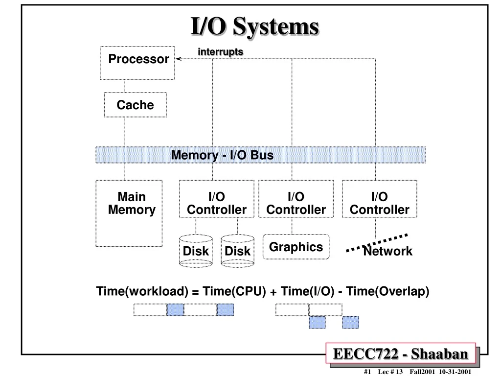
interrupts. Processor. Cache. Memory - I/O Bus. Main Memory. I/O Controller. I/O Controller. I/O Controller. Graphics. Disk. Disk. Network. Time(workload) = Time(CPU) + Time(I/O) - Time(Overlap). I/O Systems. I/O Controller Architecture. Request/response block interface

E N D
interrupts Processor Cache Memory - I/O Bus Main Memory I/O Controller I/O Controller I/O Controller Graphics Disk Disk Network Time(workload) = Time(CPU) + Time(I/O) - Time(Overlap) I/O Systems
I/O Controller Architecture Request/response block interface Backdoor access to host memory
I/O: A System Performance Perspective • CPU Performance: Improvement of 60% per year. • I/O Sub-System Performance: Limited by mechanical delays (disk I/O). Improvement less than 10% per year (IO rate per sec or MB per sec). • From Amdahl's Law: overall system speed-up is limited by the slowest component: If I/O is 10% of current processing time: • Increasing CPU performance by 10 times • 5 times system performance increase (50% loss in performance) • Increasing CPU performance by 100 times • 10 times system performance (90% loss of performance) • The I/O system performance bottleneck diminishes the benefit of faster CPUs on overall system performance.
I/O Performance Measures • Diversity: The variety of I/O devices that can be connected to the system. • Capacity: The maximum number of I/O devices that can be connected to the system. • Producer/server Model of I/O: The producer (CPU, human etc.) creates tasks to be performed and places them in a task buffer (queue); the server (I/O device or controller) takes tasks from the queue and performs them. • I/O Throughput: The maximum data rate that can be transferred to/from an I/O device or sub-system, or the maximum number of I/O tasks or transactions completed by I/O in a certain period of time • Maximized when task buffer is never empty. • I/O Latency or response time: The time an I/O task takes from the time it is placed in the task buffer or queue until the server (I/O system) finishes the task. Includes buffer waiting or queuing time. • Maximized when task buffer is always empty.
Producer-Server Model Response Time = TimeSystem = TimeQueue + TimeServer Throughput vs. Response Time
Components of A User/Computer System Transaction • In an interactive user/computer environment, each interaction or transaction has three parts: • Entry Time: Time for user to enter a command • System Response Time: Time between user entry & system reply. • Think Time: Time from response until user begins next command.
Factors Affecting I/O Processing System Performance • I/O processing computational requirements: • CPU computations available for I/O operations. • Operating system I/O processing policies/routines. • I/O Data Transfer Method used. • I/O Subsystem performance: • Raw performance of I/O devices (i.e magnetic disk performance). • IO bus capabilities. • I/O subsystem organization. • Loading level of I/O devices (queuing delay, response time). • Memory subsystem performance: • Available memory bandwidth for I/O operations.
Magnetic Disks Characteristics: • Diameter: 2.5in - 5.25in • Rotational speed: 3,600RPM-10,000 RPM • Tracks per surface. • Sectors per track: Outer tracks contain more sectors. • Recording or Areal Density: Tracks/in X Bits/in • Cost Per Megabyte. • Seek Time: The time needed to move the read/write head arm. Reported values: Minimum, Maximum, Average. • Rotation Latency or Delay: The time for the requested sector to be under the read/write head. • Transfer time: The time needed to transfer a sector of bits. • Type of controller/interface: SCSI, EIDE • Disk Controller delay or time. • Average time to access a sector of data = average seek time + average rotational delay + transfer time + disk controller overhead
Since the 1980's smaller form factor disk drives have grown in storage capacity. Today's 3.5 inch form factor drives designed for the entry-server market can store more than 75 Gbytes at the 1.6 inch height on 5 disks.
Drive areal density has increased by a factor of 8.5 million since the first disk drive, IBM's RAMAC, was introduced in 1957. Since 1991, the rate of increase in areal density has accelerated to 60% per year, and since 1997 this rate has further accelerated to an incredible 100% per year.
The price per megabyte of disk storage has been decreasing at about 40% per year based on improvements in data density,-- even faster than the price decline for flash memory chips. Recent trends in HDD price per megabyte show an even steeper reduction.
Disk Access Time Example • Given the following Disk Parameters: • Transfer size is 8K bytes • Advertised average seek is 12 ms • Disk spins at 7200 RPM • Transfer rate is 4 MB/sec • Controller overhead is 2 ms • Assume that the disk is idle, so no queuing delay exist. • What is Average Disk Access Time for a 512-byte Sector? • Ave. seek + ave. rot delay + transfer time + controller overhead • 12 ms + 0.5/(7200 RPM/60) + 8 KB/4 MB/s + 2 ms • 12 + 4.15 + 2 + 2 = 20 ms • Advertised seek time assumes no locality: typically 1/4 to 1/3 advertised seek time: 20 ms => 12 ms
I/O Data Transfer Methods • Programmed I/O (PIO): Polling • The I/O device puts its status information in a status register. • The processor must periodically check the status register. • The processor is totally in control and does all the work. • Very wasteful of processor time. • Interrupt-Driven I/O: • An interrupt line from the I/O device to the CPU is used to generate an I/O interrupt indicating that the I/O device needs CPU attention. • The interrupting device places its identity in an interrupt vector. • Once an I/O interrupt is detected the current instruction is completed and an I/O interrupt handling routine is executed to service the device.
I/O data transfer methods Direct Memory Access (DMA): • Implemented with a specialized controller that transfers data between an I/O device and memory independent of the processor. • The DMA controller becomes the bus master and directs reads and writes between itself and memory. • Interrupts are still used only on completion of the transfer or when an error occurs. • DMA transfer steps: • The CPU sets up DMA by supplying device identity, operation, memory address of source and destination of data, the number of bytes to be transferred. • The DMA controller starts the operation. When the data is available it transfers the data, including generating memory addresses for data to be transferred. • Once the DMA transfer is complete, the controller interrupts the processor, which determines whether the entire operation is complete.
Arrivals Departures Introduction to Queuing Theory • Concerned with long term, steady state than in startup: • where => Arrivals = Departures • Little’s Law: Mean number tasks in system = arrival rate x mean response time • Applies to any system in equilibrium, as long as nothing in the black box is creating or destroying tasks.
System server Queue Proc IOC Device I/O Performance & Little’s Queuing Law • Given: An I/O system in equilibrium input rate is equal to output rate) and: • Tser : Average time to service a task • Tq : Average time per task in the queue • Tsys : Average time per task in the system, or the response time, the sum of Tser and Tq • r : Average number of arriving tasks/sec • Lser : Average number of tasks in service. • Lq : Average length of queue • Lsys : Average number of tasks in the system, the sum of L q and Lser • Little’s Law states: Lsys = r x Tsys • Server utilization = u = r / Service rate = r x Tser u must be between 0 and 1 otherwise there would be more tasks arriving than could be serviced.
System server Queue Proc IOC Device A Little Queuing Theory • Service time completions vs. waiting time for a busy server: randomly arriving event joins a queue of arbitrary length when server is busy, otherwise serviced immediately • Unlimited length queues key simplification • A single server queue: combination of a servicing facility that accomodates 1 customer at a time (server) + waiting area (queue): together called a system • Server spends a variable amount of time with customers; how do you characterize variability? • Distribution of a random variable: histogram? curve?
System server Queue Proc IOC Device Avg. A Little Queuing Theory • Server spends a variable amount of time with customers • Weighted mean time m1 = (f1 x T1 + f2 x T2 +...+ fn x Tn)/F • where (F=f1 + f2...) • variance =(f1 x T12 + f2 x T22 +...+ fn x Tn2)/F – m12 • Must keep track of unit of measure (100 ms2 vs. 0.1 s2 ) • Squared coefficient of variance: C = variance/m12 • Unitless measure (100 ms2 vs. 0.1 s2) • Exponential distribution C = 1: most short relative to average, few others long; 90% < 2.3 x average, 63% < average • Hypoexponential distributionC < 1: most close to average, C=0.5 => 90% < 2.0 x average, only 57% < average • Hyperexponential distributionC > 1: further from average C=2.0 => 90% < 2.8 x average, 69% < average
System server Queue Proc IOC Device A Little Queuing Theory: Variable Service Time • Server spends a variable amount of time with customers • Weighted mean m1 = (f1xT1 + f2xT2 +...+ fnXTn)/F (F=f1+f2+...) • Squared coefficient of variance C • Disk response times C 1.5 (majority seeks < average) • Yet usually pick C = 1.0 for simplicity • Another useful value is average time must wait for server to complete task: m1(z) • Not just 1/2 x m1 because doesn’t capture variance • Can derive m1(z) = 1/2 x m1 x (1 + C) • No variance => C= 0 => m1(z) = 1/2 x m1
A Little Queuing Theory:Average Wait Time • Calculating average wait time in queue Tq • If something at server, it takes to complete on average m1(z) • Chance server is busy = u; average delay is u x m1(z) • All customers in line must complete; each avg Tser Tq = uxm1(z) + Lq x Ts er= 1/2 x ux Tser x (1 + C) + Lq x Ts er Tq = 1/2 x uxTs er x (1 + C) + r x Tq x Ts er Tq = 1/2 x uxTs er x (1 + C) + u x TqTqx (1 – u) = Ts er x u x (1 + C) /2Tq = Ts er x u x (1 + C) / (2 x (1 – u)) • Notation: r average number of arriving customers/secondTser average time to service a customeru server utilization (0..1): u = r x TserTq average time/customer in queueLq average length of queue:Lq= r x Tq
A Little Queuing Theory: M/G/1 and M/M/1 • Assumptions so far: • System in equilibrium • Time between two successive arrivals in line are random • Server can start on next customer immediately after prior finishes • No limit to the queue: works First-In-First-Out • Afterward, all customers in line must complete; each avg Tser • Described “memoryless” or Markovian request arrival (M for C=1 exponentially random), General service distribution (no restrictions), 1 server: M/G/1 queue • When Service times have C = 1, M/M/1 queueTq = Tser x u x (1 + C) /(2 x (1 – u)) = Tser x u / (1 – u) Tser average time to service a customeru server utilization (0..1): u = r x TserTq average time/customer in queue
M/M/m Queue • I/O system with Markovian request arrival rate r • A single queue serviced by m servers (disks + controllers) each with Markovian Service rate = 1/ Tser Tq = Tser x u /[m (1 – u)] u = r x Tser / m m number of servers Tser average time to service a customeru server utilization (0..1): u = r x Tser / m Tq average time/customer in queue
I/O Queuing Performance: An Example • A processor sends 10 x 8KB disk I/O requests per second, requests & service are exponentially distributed, average disk service time = 20 ms • On average: • How utilized is the disk, u? • What is the average time spent in the queue, Tq? • What is the average response time for a disk request, Tsys ? • What is the number of requests in the queue Lq? In system, Lsys? • We have: r average number of arriving requests/second = 10Tser average time to service a request = 20 ms (0.02s) • We obtain: u server utilization: u = r x Tser = 10/s x .02s = 0.2Tq average time/request in queue = Tser x u / (1 – u) = 20 x 0.2/(1-0.2) = 20 x 0.25 = 5 ms (0 .005s)Tsys average time/request in system: Tsys = Tq +Tser= 25 msLq average length of queue: Lq= r x Tq= 10/s x .005s = 0.05 requests in queueLsys average # tasks in system: Lsys = r x Tsys = 10/s x .025s = 0.25
A Little Queuing Theory: Another Example • Processor sends 20 x 8KB disk I/Os per sec, requests & service exponentially distrib., avg. disk service = 12 ms • On average: • how utilized is the disk? • What is the number of requests in the queue? • What is the average time a spent in the queue? • What is the average response time for a disk request? • Notation: r average number of arriving customers/second= 20Tser average time to service a customer= 12 msu server utilization (0..1): u = r x Tser= 20/s x .012s = 0.24Tq average time/customer in queue = Ts er x u / (1 – u) = 12 x 0.24/(1-0.24) = 12 x 0.32 = 3.8 msTsys average time/customer in system: Tsys =Tq +Tser= 15.8 msLq average length of queue:Lq= r x Tq= 20/s x .0038s = 0.076 requests in queueLsys average # tasks in system : Lsys = r x Tsys = 20/s x .016s = 0.32
A Little Queuing Theory: Yet Another Example • Suppose processor sends 10 x 8KB disk I/Os per second, squared coef. var.(C) = 1.5, avg. disk service time = 20 ms • On average: • How utilized is the disk? • What is the number of requests in the queue? • What is the average time a spent in the queue? • What is the average response time for a disk request? • Notation: r average number of arriving customers/second= 10Tser average time to service a customer= 20 msu server utilization (0..1): u = r x Tser= 10/s x .02s = 0.2Tq average time/customer in queue = Tser x u x (1 + C) /(2 x (1 – u)) = 20 x 0.2(2.5)/2(1 – 0.2) = 20 x 0.32 = 6.25 msTsys average time/customer in system: Tsys = Tq +Tser= 26 msLq average length of queue:Lq= r x Tq= 10/s x .006s = 0.06 requests in queueLsys average # tasks in system :Lsys = r x Tsys = 10/s x .026s = 0.26
Designing an I/O System • When designing an I/O system, the components that make it up should be balanced. • Six steps for designing an I/O systems are • List types of devices and buses in system • List physical requirements (e.g., volume, power, connectors, etc.) • List cost of each device, including controller if needed • Record the CPU resource demands of device • CPU clock cycles directly for I/O (e.g. initiate, interrupts, complete) • CPU clock cycles due to stalls waiting for I/O • CPU clock cycles to recover from I/O activity (e.g., cache flush) • List memory and I/O bus resource demands • Assess the performance of the different ways to organize these devices
Example: Determining the I/O BottleneckAccounting For I/O Queue Time • Assume the following system components: • 500 MIPS CPU • 16-byte wide memory system with 100 ns cycle time • 200 MB/sec I/O bus • 20 20 MB/sec SCSI-2 buses, with 1 ms controller overhead • 5 disks per SCSI bus: 8 ms seek, 7,200 RPMS, 6MB/sec • Other assumptions • All devices used to 60% capacity. • Treat the I/O system as an M/M/m queue. • Requests are assumed spread evenly on all disks. • Average I/O size is 16 KB • OS uses 10,000 CPU instr. for a disk I/O • What is the average IOPS? What is the average bandwidth? • Average response time per IO operation?
Example: Determining the I/O Bottleneck Accounting For I/O Queue Time • The performance of I/O systems is still determined by the portion with the lowest I/O bandwidth • CPU : (500 MIPS)/(10,000 instr. per I/O) x .6 = 30,000 IOPS CPU time per I/O = 10,000 / 500,000,000 = .02 ms • Main Memory : (16 bytes)/(100 ns x 16 KB per I/O) x .6 = 6,000 IOPS Memory time per I/O = 1/10,000 = .1ms • I/O bus: (200 MB/sec)/(16 KB per I/O) x .6 = 12,500 IOPS • SCSI-2: (20 buses)/((1 ms + (16 KB)/(20 MB/sec)) per I/O) = 7,500 IOPS SCSI bus time per I/O = 1ms + 16/20 ms = 1.8ms • Disks: (100 disks)/((8 ms + 0.5/(7200 RPMS) + (16 KB)/(6 MB/sec)) per I/0) x .6 = 6,700 x .6 = 4020 IOPS Tser = (8 ms + 0.5/(7200 RPMS) + (16 KB)/(6 MB/sec) = 8+4.2+2.7 = 14.9ms • The disks limit the I/O performance to r = 4020 IOPS • The average I/O bandwidth is 4020 IOPS x (16 KB/sec) = 64.3 MB/sec • Tq = Tser x u /[m (1 – u)] = 14.9ms x .6 / [100 x .4 ] = .22 ms • Response Time = Tser + Tq+ Tcpu + Tmemory + Tscsi = 14.9 + .22 + .02 + .1 + 1.8 = 17.04 ms
RAID (Redundant Array of Inexpensive Disks) • The term RAID was coined in a 1988 paper by Patterson, Gibson and Katz of the University of California at Berkeley. • In that article, the authors proposed that large arrays of small, inexpensive disks could be used to replace the large, expensive disks used on mainframes and minicomputers. • In such arrays files are "striped" and/or mirrored across multiple drives. • Their analysis showed that the cost per megabyte could be substantially reduced, while both performance and fault tolerance could be increased. • Array Reliability: Reliability of N disks = Reliability of 1 Disk ÷ N 50,000 Hours ÷ 70 disks = 700 hours • Disk system MTTF: Drops from 6 years to 1 month! • Arrays (without redundancy) too unreliable to be useful!
Basic RAID Organizations • Non-Redundant (RAID Level 0) • Mirrored (RAID Level 1) • Memory-Style ECC (RAID Level 2) • Bit-Interleaved Parity (RAID Level 3) • Block-Interleaved Parity (RAID Level 4) • Block-Interleaved Distributed-Parity (RAID Level 5) • P+Q Redundancy (RAID Level 6) • Striped Mirrors (RAID Level 10)
Manufacturing Advantages of Disk Arrays Disk Product Families Conventional: 4 disk designs 14” 3.5” 5.25” 10” High End Low End Disk Array: 1 disk design 3.5”
RAID Subsystem Organization array controller host single board disk controller host adapter manages interface to host, DMA single board disk controller control, buffering, parity logic single board disk controller physical device control single board disk controller striping software off-loaded from host to array controller no applications modifications no reduction of host performance often piggy-backed in small format devices
Non-Redundant (RAID Level 0) • RAID 0 simply stripes data across all drives (minimum 2 drives) to increase data throughput but provides no fault protection. • Sequential blocks of data are written across multiple disks in stripes, as follows: • The size of a data block, which is known as the "stripe width", varies with the implementation, but is always at least as large as a disk's sector size. • This scheme offers the best write performance since it never needs to update redundant information. • It does not have the best read performance. • Redundancy schemes that duplicate data, such as mirroring, can perform better on reads by selectively scheduling requests on the disk with the shortest expected seek and rotational delays.
Optimal Size of Data Striping Unit • Lee and Katz [1991] use an analytic model of non-redundant disk arrays to derive an equation for the optimal size of data striping unit. • They show that the optimal size of data strip-ing is equal to: • Where: • P is the average disk positioning time, • X is the average disk transfer rate, • L is the concurrency, Z is the request size, and • N is the array size in disks. • Their equation also predicts that the optimal size of data striping unit is dependent only the relative rates at which a disk positions and transfers data, PX, rather than P or X individually. Lee and Katz show that the opti-mal • striping unit depends on request size; Chen and Patterson show that this dependency can be ignored without significantly affecting performance.
Mirrored (RAID Level 1) • Utilizes mirroring or shadowing of data using twice as many disks as a non-redundant disk array. • Whenever data is written to a disk the same data is also written to a redundant disk, so that there are always two copies of the information. • When data is read, it can be retrieved from the disk with the shorter queueing, seek and rotational delays • If a disk fails, the other copy is used to service requests. • Mirroring is frequently used in database applications where availability and transaction rate are more important than storage efficiency.
Memory-Style ECC (RAID Level 2) • RAID 2 performs data striping with a block size of one bit or byte, so that all disks in the array must be read to perform any read operation. • A RAID 2 system would normally have as many data disks as the word size of the computer, typically 32. • In addition, RAID 2 requires the use of extra disks to store an error-correcting code for redundancy. • With 32 data disks, a RAID 2 system would require 7 additional disks for a Hamming-code ECC. • Such an array of 39 disks was the subject of a U.S. patent granted to Unisys Corporation in 1988, but no commercial product was ever released. • For a number of reasons, including the fact that modern disk drives contain their own internal ECC, RAID 2 is not a practical disk array scheme.
Bit-Interleaved Parity (RAID Level 3) • One can improve upon memory-style ECC disk arrays ( RAID 2) by noting that, unlike memory component failures, disk controllers can easily identify which disk has failed. Thus, one can use a single parity disk rather than a set of parity disks to recover lost information. • As with RAID 2, RAID 3 must read all data disks for every read operation. • This requires synchronized disk spindles for optimal performance, and works best on a single-tasking system with large sequential data requirements. An example might be a system used to perform video editing, where huge video files must be read sequentially.
Block-Interleaved Parity (RAID Level 4) • RAID 4 is similar to RAID 3 except that blocks of data are striped across the disks rather than bits/bytes. • Read requests smaller than the striping unit access only a single data disk. • Write requests must update the requested data blocks and must also compute and update the parity block. • For large writes that touch blocks on all disks, parity is easily computed by exclusive-or’ing the new data for each disk. • For small write requests that update only one data disk, parity is computed by noting how the new data differs from the old data and apply-ing those differences to the parity block. • This can be an important performance improvement for small or random file access (like a typical database application) if the application record size can be matched to the RAID 4 block size.
Block-Interleaved Distributed-Parity (RAID Level 5) • The block-interleaved distributed-parity disk array eliminates the parity disk bottleneck present in RAID 4 by distributing the parity uniformly over all of the disks. • An additional, frequently overlooked advantage to distributing the parity is that it also distributes data over all of the disks rather than over all but one. • RAID 5 has the best small read, large read and large write performance of any redundant disk array. • Small write requests are somewhat inefficient compared with redundancy schemes such as mirroring however, due to the need to perform read-modify-write operations to update parity.
RAID-5: Small Write Algorithm 1 Logical Write = 2 Physical Reads + 2 Physical Writes D0 D1 D2 D0' D3 P old data new data old parity (1. Read) (2. Read) XOR + + XOR (3. Write) (4. Write) D0' D1 D2 D3 P' Problems of Disk Arrays: Small Writes
P+Q Redundancy (RAID Level 6) • An enhanced RAID 5 with stronger error-correcting codes used . • One such scheme, called P+Q redundancy, uses Reed-Solomon codes, in addition to parity, to protect against up to two disk failures using the bare minimum of two redundant disks. • The P+Q redundant disk arrays are structurally very similar to the block-interleaved distributed-parity disk arrays (RAID 5) and operate in much the same manner. • In particular, P+Q redundant disk arrays also perform small write opera-tions using a read-modify-write procedure, except that instead of four disk accesses per write requests, P+Q redundant disk arrays require six disk accesses due to the need to update both the ‘P’ and ‘Q’ information.
Increasing Logical Disk Addresses D0 D1 D2 D3 P A logical write becomes four physical I/Os Independent writes possible because of interleaved parity Reed-Solomon Codes ("Q") for protection during reconstruction D4 D5 D6 P D7 D8 D9 P D10 D11 D12 P D13 D14 D15 Stripe P D16 D17 D18 D19 Targeted for mixed applications Stripe Unit D20 D21 D22 D23 P . . . . . . . . . . . . . . . Disk Columns RAID 5/6: High I/O Rate Parity
RAID 10 (Striped Mirrors) • RAID 10 (also known as RAID 1+0) was not mentioned in the original 1988 article that defined RAID 1 through RAID 5. • The term is now used to mean the combination of RAID 0 (striping) and RAID 1 (mirroring). • Disks are mirrored in pairs for redundancy and improved performance, then data is striped across multiple disks for maximum performance. • In the diagram below, Disks 0 & 2 and Disks 1 & 3 are mirrored pairs. • Obviously, RAID 10 uses more disk space to provide redundant data than RAID 5. However, it also provides a performance advantage by reading from all disks in parallel while eliminating the write penalty of RAID 5.
RAID Levels Comparison:Throughput Per Dollar Relative to RAID Level 0.
RAID Levels Comparison:Throughput Per Dollar Relative to RAID Level 0.