Download
1 / 18
180 likes | 304 Views
9.4 Random Numbers from Various Distributions. Distributions. A distribution of numbers is a description of the portion of times each possible outcome or range of outcomes occurs on average. A histogram is a display of a given distribution.

E N D
Distributions • A distribution of numbers is a description of the portion of times each possible outcome or range of outcomes occurs on average. • A histogram is a display of a given distribution. • In a uniform distribution all outcomes are equally likely.
Uniform Distribution: Hypothetical Consider a hospital at which there are an average of 100 births per day:
Discrete vs. Continuous Distributions • A discrete distribution is one in which the values (x, y axis values) are discrete (countable, finite in number). • A continuous distribution is one in which the values (x, y axis values) are continuous (not countable). • In practice, we can model continuous distributions discretely by binning….
Probability Density Function • For a discrete distribution, a probability density function (or density function or probability function) tells us the probability of occurrence of its input. • For a continuous distribution, the PDF indicates the probability that a given outcome falls inside a specific range of values.
Probability Density Function • For a discrete distribution, we just report the value at that bin. • For a continuous distribution, we integrate between the ends of the interval (Fundamental Theorem of Calculus), or approximate that using numerical methods (Euler, RK4)
Generating Random Numbers in Non-Uniform Distributions Imagine a biased roulette wheel for picking events (outcomes) e1, e2, …. e2 .60 .68 .78 1.0 e3 e1 e3 e4 e2 e1 10% 22% 8% 60% e4
Generating Random Numbers in Non-Uniform Distributions Given probabilities p1, p2, …. for events e1, e2, …. : Generate rand, a uniform random floating-point number in [0,1); that is, from zero up to but excluding 1. If rand < p1 then use e1 Else if rand < p1+p2 then use e2 … Else if rand < p1+p2+…+pn-1+then use en-1 Else use en
Carl Friedrich Gauss(1777-1855) Normal (Gaussian) Distributions Gauss Gerling Plücker Klein Story Lefschetz Tucker Minsky Winston Waltz Pollack Levy Y’all
Normal (Gaussian) Distributions • The standard deviation sof a set of values is their average difference from their mean m. • In a normal distribution (so-called because it is so common) 68.3% of the values are within ±s (one standard deviation) of m; 95.5% are within ±2s; and 99.7% are within ±3s. I.e., extreme values are rare. • Where do these strange percentages come from?
Normal (Gaussian) Distributions • Normal distribution has probability density function • Random number generators typically use m = 0, s = 1, so this simplifies to
Normal (Gaussian) Distributions • is a constant, so the shape is given by ; i.e., something that reaches a peak at x = 0 and tapers off rapidly as x grows positive or negative: • How can we build such a distribution from our uniformly-distributed random numbers?
Box-Muller-Gauss Method for Normal Distributions with Mean m And Standard Deviation s • Start with two uniform random numbers: • a in [0,2p) • rand in [0,1) • Then compute • Obtain two normally distributed numbers • b sin(a) + m • b cos(a) + m
Exponential Distributions • Common pattern is exponentially decaying PDF, also called 1/f noise (a.k.a. pink noise) • noise = random • f = frequency; i.e., larger events are less common • pink because uniform distribution is “white” (white light = all frequencies) • “Universality” is a current topic of controversy (Shalizi 2006)
Exponential Method for PDF |r|ertwhere t>0, r<0 • Start with uniform random rand in [0,1) • Compute ln(rand)/r • E.g., ln(rand) / (-2) gives 1/fnoise
Rejection Method • To get random numbers in interval [a, b) for distribution f(x): • Generate randInterval, a uniform random number in [a, b) • Generate randUpperBound, a uniform random number in [0, upper bound for f ) • If f(randInterval) > randUpperBound then use randInterval • E.g. for normal distribution with m = 0, s = 1, randInterval = approx. [-3,3) upperBound = 1