Download
1 / 6
60 likes | 118 Views
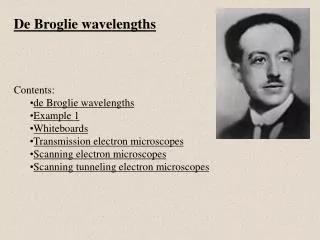
EXAMPLE 2.2 OBJECTIVE Determine the de Broglie wavelength of a particle. Consider an electron traveling at a velocity of 10 7 cm/s = 10 5 m/s. Solution The momentum is given by p = mv = (9.11 10 -31 )(10 5 ) = 9.11 10 -26 kg-m/s Then the de Broglie wavelength is or

E N D
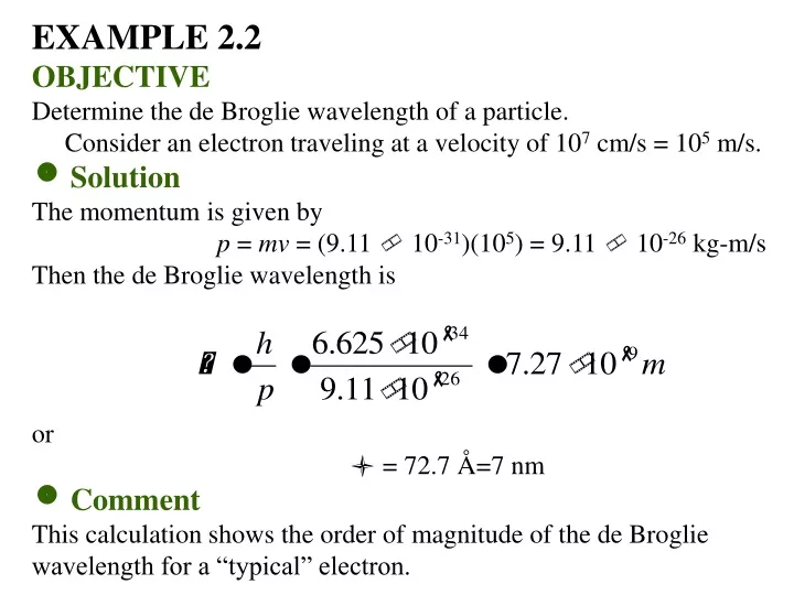
EXAMPLE 2.2 • OBJECTIVE • Determine the de Broglie wavelength of a particle. • Consider an electron traveling at a velocity of 107 cm/s = 105 m/s. • Solution The momentum is given by p = mv = (9.11 10-31)(105) = 9.11 10-26 kg-m/s Then the de Broglie wavelength is or = 72.7 Å=7 nm • Comment This calculation shows the order of magnitude of the de Broglie wavelength for a “typical” electron.
EXAMPLE 2.3 • OBJECTIVE • Determine the first three allowed electron energies in the hydrogen atom. • Solution The mass of an electron is m0 = 9.11 10-31 kg and the permittivity of free apace is o = 8.85 10-12 F/m. The modified Planck’s constant is The first energy level, from Equation (2.11) for n = 1, is The second and third allowed energy levels are determined by setting n = 2 and n = 3. We find E2 = -3.39 eV and E3 = -1.51 eV • Comment The first allowed energy level corresponds to the given value of ionization energy of hydrogen. The classical representation of the first three energy levels is shown in Figure 2.3. The energy of the electron increases (becomes less negative) as the orbit of the electron bexomes larger.
EXAMPLE 2.5 • OBJECTIVE • Find the density of states per unit volume over a particular energy range. • Consider the density of states for a free electron given by Equation (2.26). Calculate the density of states for a fess electro given by Equation (2.26). Calculate the density of states per unit volume with energies between zero and 1 eV. • Solution The volume density of quantum states, using Equation (2.26), can be found from or The density of states is now or • Comment The density of quantum states is typically a large number. An effective density of states in a semiconductor, as we will see in Chapter 3, is also a large number but is usually less than the density of atoms in the semiconductor crystal.
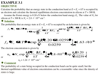
EXAMPLE 2.6 • OBJECTIVE • Determine the probability that an energy state above EF is occupied by an electron. • Let T = 300 K. Determine the probability that an energy level 3kT above the Fermi energy level is occupied by an electron. (Assume that such an energy level is allowed.) • Solution From Equation (2.29), we ca\n write which becomes • Comment At energies above EF the probability of a state being occupied by an electron can become significantly less than unity, or the ratio of electrons to available quantum states can be quite small.
EXAMPLE 2.7 • OBJECTIVE • Find the temperature at which there is a 1 percent probability that an energy state is empty. • assume that the Fermi energy level for a particular material is 6.25 eV and that the electrons in this material follow the Fermi-Dirac distribution function. Calculate the temperature at which there is a 1 percent probability that a state 0.30 eV below the Fermi energy level will not contain an electron. • Solution The probability that a state is empty is Then, We find that kT = 0.06529 eV. Which corresponds to a temperature of T = 756 K. • Comment The Fermi probability function is a strong function of temperature.
EXAMPLE 2.8 • OBJECTIVE • Determine the energy at which the Boltzmann approximation can be considered valid. • Calculate the energy, in terms of kT and EF, at which the difference between the Boltzmann approximation and the Fermi-Dirac function is 5 percent of the Fermi function. • Solution We can write If we multiply both the numerator and denominator by the 1 + exp ( ) function, we have which becomes Or • Comment As seen in this example and in Figure 2.26, the E – EF >> kT notation is somewhat misleading. The Maxwell-Boltzmann and Fermi-Dirac functions are within 5 percent of each other when E –EF > 3 kT.