Download

1 / 31
310 likes | 470 Views
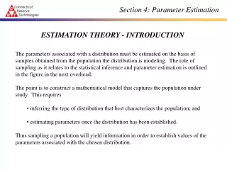
Parameter Estimation. Estimation of the Mean. Suppose y 1 ………. y n are independent and identically distributed. The method of moments estimator (and least squares estimator) of the population mean μ is given by the sample mean. Also. where σ is the population standard deviation.

E N D
Parameter Estimation Estimation of the Mean
Suppose y1 ………. yn are independent and identically distributed. The method of moments estimator (and least squares estimator) of the population mean μ is given by the sample mean Also where σ is the population standard deviation
It can be shown that The relation comes from the Central Limit Theorem and usually holds good in practice for all but the smallest values of n. Confidence intervals for the population mean can be calculated. (often by usingsample mean +/- 2 standard errors)
However,σ usually needs to be estimated by the sample standard deviation and this introduces an additional degree of uncertainty which should lead to wider confidence intervals.
However,σ usually needs to be estimated by the sample standard deviation and this introduces an additional degree of uncertainty which should lead to wider confidence intervals. When the population distribution is approximately normal we can make an appropriate correction by replacing the normal distribution with the t distribution with n-1 degrees of freedom. Otherwise a greater correction is ideally required.
Example: Failures Data The numbers of operating hours between successive failures of the air conditioning equipment aboard an aircraft were as follows: 413 14 58 37 100 65 9 169 447 184 36 201 118 34 31 18 18 67 57 62 7 22 34 The data are also available as the R vector failures. We have n = 23 observations.
The data are clearly very positively skewed so an exponential Q-Q plot is carried out.
The graph suggests that they might reasonably be modelled by an Exp( μ-1) distribution (exponential mean μ ), corresponding to a memoryless property in the failure times. From the plot, a resistant estimate of μ would appear to be about 80, but it is difficult to make any (graphical) assessment of uncertainty.
We now wish to find an estimate of the population mean, μ. Let μ be the sample mean.
We can also work out the standard error S.E. is given by σ/√n so is 119.2897/√23 This calculates as 24.87
A 95% confidence interval can be calculated by the usual methods or obtained on R. Since the population standard deviation has been estimated from the sample and the sample size is reasonably small, the t distribution is appropriate.
So the 95% confidence interval is [44.11,147.28]. This should really be widened a little bit to allow for non-normality of the population distribution.
Estimation of the Median Sometimes it can be more useful to look at the population MEDIAN rather than mean. A possible estimator of this is given by the sample median, m. Here, at least when n is moderately large, where f(m) is the density of the underlying distribution at the median m.
For a normally distributed N(μ, σ) population, the sample median has standard error 1.253σ/√n, and so is a less efficient estimator of μ than the sample mean. However, for longer-tailed distributions, the sample median is a more efficient estimator of location than the sample mean. This is a closely related to the fact that the sample median is a resistant estimator. We will use the median in the “failures” example.
Example: Estimation of Median for Failures Data We can estimate the population median from the sample median which has a value of 57. We need to ask, though, how accurate is this estimate and can we use it to construct a confidence interval for m?
We could use the formula for the standard error quoted earlier to calculate confidence intervals but the sample size is not very large. We instead use bootstrap estimation to answer these questions.
Bootstrap estimation is a fairly general technique for making assessments of uncertainty about estimators. It typically requires the use of simulation. What we would like is the sampling distribution of m - m, giving the variation of the sample median about the population median. ^
However, this requires knowledge of the (unknown) underlying population distribution. We therefore substitute for the population distribution by using instead the empirical distribution of the data (the bootstrap).
Suppose this empirical distribution has median m*. Let the random variable m* denote the sample median of a random sample (independent identically distributed observations) of size 23 from this empirical distribution. Then we would expect that the sampling distribution of m* - m* should be very close to that of m - m. ^ ^
Now let us study the distribution of of m*- m*. Since we know the value of m* (57), it is just a case of looking at m*. We will use simulation and set up an R vector called ms of size 1000 and use it to store the results of 1000 simulations of m*. First consider the command sample. ^ ^ ^
Recall that each component of ms is the median of a random sample of size 23, obtained by sampling with replacement from failures. Hence the variability in ms is much less than the variability in failures itself. Typing qqnorm(ms) produces the normal Q-Q plot for the distribution of ms.
This distribution is not particularly normal, so the earlier theory for the sampling distribution of the median would not have been very good here. A reasonable 95% confidence interval, more formally a 95% percentile interval, for the original population median m is given by [Qe(0.025), Qe(0.975)], where Qe is the empirical quantile function of the bootstrap simulations ms of m ^
So that (34,67) is a reasonable confidence interval for m. Again, this confidence interval should be widened a little to allow for the approximation involved in using the empirical distribution of the data.
Failures data - further discussion. If we assume that the population distribution is Exp( μ-1), then for the population median, m, we have m = μ ln 2.
Failures data - further discussion. If we assume that the population distribution is Exp( μ-1), then for the population median, m, we have m = μ ln 2. It follows that we can also obtain an estimate of the population mean, μ, from an estimate of m. In particular the 95% confidence interval for m of (34, 67) obtained above translates into a 95% confidence interval for μ of (49.1, 96.7).
This should be compared with that obtained earlier by estimation based on the sample mean (44,147). However, no allowance is made here for the uncertainty involved in the exponential assumption.