Download

1 / 21
300 likes | 780 Views
Water Quality. Water Resources Planning and Management Daene C. McKinney. Water Quality Management. Critical component of overall water management in a basin Water bodies serve many uses, including Transport and assimilation of wastes

E N D
Water Quality Water Resources Planning and Management Daene C. McKinney
Water Quality Management • Critical component of overall water management in a basin • Water bodies serve many uses, including • Transport and assimilation of wastes • Assimilative capacities of water bodies can be exceeded WRT intended uses • Water quality management measures • Standards • Minimum acceptable levels of ambient water quality • Actions • Insure pollutant load does not exceed assimilative capacity while maintaining quality standards • Treatment
Water Quality Management Process • Identify • Problem • Indicators • Target Values • Assess source(s) • Determine linkages • Sources Targets • Allocate permissible loads • Monitor and evaluate • Implement
Water Quality Example • W1,W2 = Pollutant loads (kg/day) • x1, x2 = Waste removal efficiencies (%) • P2max, P3max = Water quality standards (mg/l) • P2, P3 = Concentrations (mg/l) • Q1, Q2,Q3= Flows (m3/sec) • a12, a13, a23, = Transfer coefficients
Water Quality Example • Cost of treatment at 1 greater than cost at 2 (bigger waste load at 1) • Marginal cost at 1 greater than marginal cost at 2, c1 > c2 for same level of treatment
Water Quality Example Cost of treatment at 1 >= cost at 2 marginal cost at 1, c1, >= marginal cost at 2, c1, for the same amount of treatment.
Example • Irrigation project • 1800 acre-feet of water per year • Decision variables • xA = acres of Crop A to plant? • xB = acres of Crop B to plant? 1,800 acre feet = 2,220,267 m3 400 acre = 1,618,742 m2
Example xA< 400 xA> 0 10 8 xB< 600 6 xB (hundreds acres) 4 3xA +2 xB < 1800 2 xB > 0 2 4 6 8 10 xA (hundreds acres)
Example xA< 400 xA> 0 10 Z=3600=300xA +500xB (200, 600) 8 xB< 600 6 xB (hundreds acres) Z=2000=300xA +500xB 4 Z=1000=300xA +500xB 2 xB > 0 2 4 6 8 10 xA (hundreds acres)
GAMS Code POSITIVE VARIABLES xA, xB; VARIABLES obj; EQUATIONS objective, xAup, xBup, limit; objective.. obj =E= 300*xA+500*xB; xAup.. xA =L= 400.; xBup.. xB =L= 600.; limit.. 3*xA+2*xB =L= 1800; MODEL Calibrate / ALL /; SOLVE Calibrate USING LP MAXIMIZING obj; Display xA.l; Display xB.l; Marginal, Lagrange multiplier, shadow price, dual variable
GAMS Output LOWER LEVEL UPPER MARGINAL ---- EQU objective . . . 1.000 ---- EQU xAup -INF 200.000 400.000 . ---- EQU xBup -INF 600.000 600.000 300.000 ---- EQU limit -INF 1800.000 1800.000 100.000 LOWER LEVEL UPPER MARGINAL ---- VAR xA . 200.000 +INF . ---- VAR xB . 600.000 +INF . ---- VAR obj -INF 3.6000E+5 +INF . Marginal
Marginals • Marginal for a constraint = Change in the objective per unit increase in RHS of that constraint. • i.e., change xB • Objective = 360,000 • Marginal for constraint = 300 • Expect new objective value = 360,300
New Solution LOWER LEVEL UPPER MARGINAL ---- EQU objective . . . 1.000 ---- EQU xAup -INF 199.333 400.000 . ---- EQU xBup -INF 601.000 601.000 300.000 ---- EQU limit -INF 1800.000 1800.000 100.000 LOWER LEVEL UPPER MARGINAL ---- VAR xA . 199.333 +INF . ---- VAR xB . 601.000 +INF . ---- VAR obj -INF 3.6030E+5 +INF . Note: Adding 1 unit to xB adds 300 to the objective, but constraint 3 says and this constraint is “tight” (no slack) so it holds as an equality, therefore xA must decrease by 1/3 unit for xB to increase by a unit.
Unbounded Solution Take out constraints 3 and 4, objective can Increase without bound xA< 400 xA> 0 10 unbounded 8 6 xB (hundreds acres) 4 2 xB > 0 2 4 6 8 10 xA (hundreds acres)
Infeasibility Change constraint 4 to >= 3000, then no intersection of constraints exists and no feasible solution can be found xA< 400 xA> 0 10 3xA +2 xB > 3000 8 xB< 600 6 xB (hundreds acres) 4 2 xB > 0 2 4 6 8 10 xA (hundreds acres)
Multiple Optima xA< 400 xA> 0 10 Infinite solutions on this edge 8 Z=1800=300xA +200xB xB< 600 6 Change objective coefficient to 200, then objective has same slope as constraint and infinite solutions exist xB (hundreds acres) 4 3xA +2 xB < 1800 2 xB > 0 2 4 6 8 10 xA (hundreds acres)