Download
1 / 30
300 likes | 541 Views
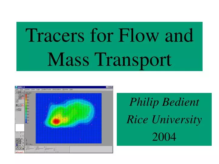
Tracers for Flow and Mass Transport. Philip Bedient Rice University 2004. Transport of Contaminants. Transport theory tries to explain the rate and extent of migration of chemicals from known source areas Source concentrations and histories must be estimated and are often not well known

E N D
Tracers for Flow and Mass Transport Philip Bedient Rice University 2004
Transport of Contaminants • Transport theory tries to explain the rate and extent of migration of chemicals from known source areas • Source concentrations and histories must be estimated and are often not well known • Velocity fields are usually complex and can change in both space and time • Dispersion causes plumes to spread out in x and y • Some plumes have buoyancy effects as well
What Drives Mass Transport: Advection and Dispersion • Advection is movement of a mass of fluid at the average seepage velocity, called plug flow • Hydrodynamic dispersion is caused by velocity variations within each pore channel and from one channel to another • Dispersion is an irreversible phenomenon by which a miscible liquid (the tracer) that is introduced to a flow system spreads gradually to occupy an increasing portion of the flow region
Advection and Dispersionin a Soil Column Source Spill t = 0 Conc = 100 mg/L Longitudinal Dispersion t = t1 n = Vv/Vt porosity Advection t = t1 C t
Contaminant Transport in 1-D Fx + (dFx/dx) dx Fx y z Fx = total mass per area transported in x direction Fy = total mass per area transported in y direction Fz = total mass per area transported in z direction
Substituting in Fx for the x direction only yields Accumulation Dispersion Advection C = Concentration of Solute [M/L3] D = Dispersion Coefficient [L2/T] V = Velocity in x Direction [L/T]
2-D Computed Plume Map Advection and Dispersion
Analytical 1-D, Soil Column • Developed by Ogata and Banks, 1961 • Continuous Source • C = Co at x = 0 t > 0 • C (x, ) = 0 for t > 0
Error Function - Tabulated Fcn Erf (0) = 0 Erf (3) = 1 Erfc (x) = 1 - Erf (x) Erf (–x) = – Erf (x) Erf x
Contaminant Transport Equation C = Concentration of Solute [M/L3] DIJ = Dispersion Coefficient [L2/T] B = Thickness of Aquifer [L] C’ = Concentration in Sink Well [M/L3] W = Flow in Source or Sink [L3/T] n = Porosity of Aquifer [unitless] VI = Velocity in ‘I’ Direction [L/T] xI = x or y direction
Analytical Solutions of Equations Closed form solution, C = C ( x, y, z, t) • Easy to calculate, can often be done on a spreadsheet • Limited to simple geometries in 1-D, 2-D, or 3-D • Limited to simple sources such as continuous or instantaneous or simple combinations • Requires aquifer to be homogeneous and isotropic • Error functions (Erf) or exponentials (Exp) are usually involved
Numerical Solution of Equations Numerically -- C is approximated at each point of a computational domain (may be a regular grid or irregular) • Solution is very general • May require intensive computational effort to get the desired resolution • Subject to numerical difficulties such as convergence problems and numerical dispersion • Generally, flow and transport are solved in separate independent steps (except in density-dependent or multi-phase flow situations)
Domenico and Schwartz (1990) • Solutions for several geometries (listed in Bedient et al. 1999, Section 6.8). • Generally a vertical plane, constant concentration source. Source concentration can decay. • Uses 1-D velocity (x) and 3-D dispersion (x,y,z) • Spreadsheets exist for solutions. • Dispersion = axvx, where ax is the dispersivity (L) • BIOSCREEN (1996) is handy tool that can be downloaded.
BIOSCREEN Features • Answers how far will a plume migrate? • Answers How long will the plume persist? • A decaying vertical planar source • Biological reactions occur until the electron acceptors in GW are consumed • First order decay, instantaneous reaction, or no decay • Output is a plume centerline or 3-D graphs • Mass balances are provided
Domenico and Schwartz (1990) y Plume at time t Vertical Source x z
Domenico and Schwartz (1990) For planar source from -Y/2 to Y/2 and 0 to Z Y Flow x Z Geometry
Instantaneous Spill in 2-D Spill source C0released at x = y = 0, v = vx First order decay l and release area A 2-D Gaussian Plume moving at velocity V
Breakthrough Curves 2 dimensional Gaussian Plume
Tracer Tests • Aids in the estimation of average hydraulic conductivity between sampling locations • Involves the introduction of a non-reactivechemical species of knownconcentration • Average seepage velocities can be calculated from resulting curves of concentration vs. time using Darcy’s Law
What can be used as a tracer? • An ideal tracer should: 1. Be susceptible to quantitative determination 2. Be absent from the natural water 3. Not react chemically or be absorbed 4. Be safe in drinking water 5. Be inexpensive and available • Examples: • Bromide, Chloride, Sulfates • Radioisotopes • Water-soluble dyes
Hour 14 Hour 43 Hour 85 Hour 8 Hour 30 Hour 55 Hour 79
Outlet 13 11 9 10 14 12 1 4 5 2 3 6 7 8 24 21 23 22 25 26 28 27 17 15 19 20 16 18 Inlet Bromide Tracer Front - ECRS Black Arrows @ t= 40 hrs Red Arrows @ t= 85 hrs
New Experimental Tank • 5000 mg/L Bromide tracer in advance of ethanol test • Pumped into 6 wells for 7 hour injection period • Pumping rate of 360 mL/min was maintained • Background water flow rate was 900-1000 mL/min
PLAN VIEW OF TANK Flow
July 2004 New Tank prior to 95E test (5.5 ft to 9.5 ft down tank)