Download

1 / 37
370 likes | 521 Views
Power and Sample Size. Shaun Purcell & Danielle Posthuma Twin Workshop March 2002. Aims of Session. Introduce concept of power and errors in inference Practical 1 : Using probability distribution functions to calculate power Power in the classical ACE twin study

E N D
Power and Sample Size Shaun Purcell & Danielle Posthuma Twin Workshop March 2002
Aims of Session • Introduce concept of power and errors in inference • Practical 1 : Using probability distribution functions to calculate power • Power in the classical ACE twin study • Practical 2 : using Mx to calculate power • Practical 3 : Monte-Carlo simulation
YES NO Test statistic YES OR NO decision-making : significance testing Power primer • Statistics (e.g. chi-squared, z-score) are continuous measures of support for a certain hypothesis Inevitably leads to two types of mistake : false positive (YES instead of NO) (Type I) false negative (NO instead of YES) (Type II)
Hypothesis testing • Null hypothesis : no effect • A ‘significant’ result means that we can reject the null hypothesis • A ‘nonsignificant’ result means that we cannot reject the null hypothesis
Statistical significance • The ‘p-value’ • The probability of a false positive error if the null were in fact true • Typically, we are willing to incorrectly reject the null 5% or 1% of the time (Type I error)
Misunderstandings • p - VALUES • that the p value is the probability of the null hypothesis being true • that very low p values mean large and important effects • NULL HYPOTHESIS • that nonrejection of the null implies its truth
Limitations • IF A RESULT IS SIGNIFICANT • leads to the conclusion that the null is false • BUT, this may be trivial • IF A RESULT IS NONSIGNIFICANT • leads only to the conclusion that it cannot be concluded that the null is false
Alternate hypothesis • Neyman & Pearson (1928) • ALTERNATE HYPOTHESIS • specifies a precise, non-null state of affairs with associated risk of error
Sampling distribution if H0 were true Sampling distribution if HA were true Critical value P(T) T
Type I error at rate Nonsignificant result Type II error at rate Significant result STATISTICS Nonrejection of H0 Rejection of H0 H0 true R E A L I T Y HA true POWER =(1- )
Power • The probability of rejection of a false null-hypothesis • depends on • - the significance crtierion () • - the sample size (N) • - the effect size (NCP) “The probability of detecting a given effect size in a population from a sample of size N, using significance criterion ”
Critical value Impact of alpha P(T) T
Critical value Impact of effect size, N P(T) T
Applications • POWER SURVEYS / META-ANALYSES • - low power undermines the confidence that can be placed in statistically significant results • EXPERIMENTAL DESIGN • - avoiding false positives vs. dealing with false negatives • MAGNITUDE VS. SIGNIFICANCE • - highly significant very important • INTERPRETING NONSIGIFICANT RESULTS • - nonsignficant results only meaningful if power is high
Practical Exercise 1 • Calculation of power for simple case-control study. • DATA : frequency of risk factor in 30 cases and 30 controls • TEST : 2-by-2 contingency table : chi-squared • (1 degree of freedom)
Step 1 : determine expected chi-squared • Hypothetical risk factor frequencies • Case Control • Risk present 20 10 • Risk absent 10 20 Chi-squared statistic = 6.666
Step 2. Determine the critical value for a given type I error rate, - inverse central chi-squared distribution P(T) Critical value T
Step 3. Determine the power for a given critical value and non-centrality parameter - non-central chi-squared distribution P(T) Critical value T
2. Calculate power (Non-central 2) Crit. value Expected NCP Calculating Power 1. Calculate critical value (Inverse central 2) Alpha 0 (under the null)
3.84146 6.63489 10.82754 • http://workshop.colorado.edu/~pshaun/ • df = 1 , NCP = 0 • X • 0.05 • 0.01 • 0.001
0.73 0.50 0.24 Determining power • df = 1 , NCP = 6.666 • X Power • 0.05 3.84146 • 0.01 6.6349 • 0.001 10.827
Exercise 1 • Calculate power (for the 3 levels of alpha) if sample size were two times larger (assume proportions remain constant) ? • Hint: the NCP is a linear function of sample size, and will also be two times larger
Answers • df = 1 , NCP = 13.333 • X Power • 0.05 3.84146 • 0.01 6.6349 • 0.001 10.827 • nb. Stata : di 1-nchi(df,NCP,invchi(df,)) 0.95 0.86 0.64
Estimating power for twin models • The power to detect, e.g., common environment Expected covariance matrices are calculated under the alternate model : Fit model to data with value of interest fixed to null value, e.g. c = 0 A C E A C E a c e a’ 0 e’ Twin 1 Twin 1 NCP = -2LLSUB
Using power.mx script • Model A C E • 1 30% 20% 50% • 2 0% 20% 80% • (350 MZ pairs, 350 DZ pairs) • Model Power to detect C • Alpha 0.05 0.01 • 1 • 2 0.51 0.28 0.41 0.20
Using power.mx script • Qu. You observe MZ and DZ correlations of 0.8 and 0.5 respectively, in 100 MZ and 100 DZ twin pairs. What is the power to detect an additive genetic effect, with a type I error rate of 1 in 1000?
Absolute ACE effects • Power to detect : • A C E A C • 0.1 0.1 0.8 0.02 0.02 • 0.2 0.2 0.6 0.06 0.09 • 0.3 0.3 0.4 0.29 0.32 • 0.4 0.4 0.2 0.95 0.79 • 150 MZ twins, 150 DZ twins, = 0.01
Relative ACE effects • Power to detect : • A C E A C • 0.2 0.2 0.6 0.06 0.09 • 0.2 0.0 0.8 0.57 • 0.0 0.2 0.8 0.82 • 150 MZ twins, 150 DZ twins, = 0.01
Sample Size • NMZ NDZ A C • 150 150 0.83 0.53 • 250 250 0.98 0.86 • 350 350 1.00 0.96 • 500 500 1.00 0.99 • A:C:E = 2:2:1, = 0.001
Relative MZ and DZ sample N • NMZ NDZ A C • 150 150 0.83 0.53 • 500 500 1.00 0.99 • 500 150 0.99 0.56 • 150 500 0.95 0.99 • A:C:E = 2:2:1, = 0.001
Increasing power • Increase sample size • Increase • Multivariate analysis • Adding other family members
Adding other siblings • Power compared to twins only design • (keeping total # individuals constant) • Power to detect • A C D • + 1 sibling + ++ ++ • + 2 siblings - ++ ++
Monte-Carlo simulation • Instead of calculating expected NCP under population parameter values, simulate multiple randomly-sampled datasets • Perform test on each dataset • Due to random sampling variation, the effect will not always be detectable • The proportion of significant results Power
Critical value Critical value Expected NCP P(T) T P(T) T
More importantly... • Meike says … • “people are going skiing Saturday and all are welcome to join”