Download
1 / 52
530 likes | 712 Views
Extending ArcGIS using programming. David Tarboton. Why Programming. Automation of repetitive tasks (workflows) Implementation of functionality not available (programming new behavior). ArcGIS programming entry points. Model builder Python scripting environment

E N D
Extending ArcGIS using programming David Tarboton
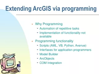
Why Programming • Automation of repetitive tasks (workflows) • Implementation of functionality not available (programming new behavior)
ArcGIS programming entry points • Model builder • Python scripting environment • ArcObjects library (for system language like C++, .Net) • Open standard data formats that anyone can use in programs (e.g. shapefiles, geoTIFF, netCDF)
Three Views of GIS Geodatabase view: Structured data sets that represent geographic information in terms of a generic GIS data model. Geovisualization view: A GIS is a set of intelligent maps and other views that shows features and feature relationships on the earth's surface. "Windows into the database" to support queries, analysis, and editing of the information. Geoprocessing view: Information transformation tools that derive new geographic data sets from existing data sets. adapted from www.esri.com
http://resources.arcgis.com/en/help/main/10.1/002w/002w00000001000000.htmhttp://resources.arcgis.com/en/help/main/10.1/002w/002w00000001000000.htm
An example – time series interpolation Soil moisture at 8 sites in field Hourly for a month ~ 720 time steps What is the spatial pattern over time Data from ManalElarab
How to use in ArcGIS • Time series in Excel imported to Object class in ArcGIS • Joined to Feature Class (one to many)
Time enabled layer with 4884 records that can be visualized using time slider
But what if you want spatial fields • Interpolate using spline or inverse distance weight at each time step • Analyze resulting rasters • 30 days – 720 hours ??? • A job for programming
The program workflow • Set up inputs • Get time extents from the time layer • Create a raster catalog (container for raster layers) • For each time step • Query and create layer with data only for that time step • Create raster using inverse distance weight • Add raster to raster catalog • Add date time field and populate with time values
I used PyScripter(as suggested by an ESRI programmer http://blogs.esri.com/esri/arcgis/2011/06/17/pyscripter-free-python-ide/) http://code.google.com/p/pyscripter/
This shows the reading of time parameters and creation of raster catalog
Terrain Analysis Using Digital Elevation Models (TauDEM) David Tarboton1, Dan Watson2, Rob Wallace3 1Utah Water Research Laboratory, Utah State University, Logan, Utah 2Computer Science, Utah State University, Logan, Utah 3US Army Engineer Research and Development Center, Information Technology Lab, Vicksburg, Mississippi http://hydrology.usu.edu/taudemdtarb@usu.edu This research was funded by the US Army Research and Development Center under contracts number W9124Z-08-P-0420 and W912HZ-09-P-0338
TauDEM - Channel Network and Watershed Delineation Software • Pit removal (standard flooding approach) • Flow directions and slope • D8 (standard) • D (Tarboton, 1997, WRR 33(2):309) • Flat routing (Garbrecht and Martz, 1997, JOH 193:204) • Drainage area (D8 and D) • Network and watershed delineation • Support area threshold/channel maintenance coefficient (Standard) • Combined area-slope threshold (Montgomery and Dietrich, 1992, Science, 255:826) • Local curvature based (using Peuker and Douglas, 1975, Comput. Graphics Image Proc. 4:375) • Threshold/drainage density selection by stream drop analysis (Tarboton et al., 1991, Hyd. Proc. 5(1):81) • Other Functions: Downslope Influence, Upslope Dependence, Wetness index, distance to streams, Transport limited accumulation • Developed as C++ command line executable functions • MPICH2 used for parallelization (single program multiple data) • Relies on other software for visualization (ArcGIS Toolbox GUI)
Website and Demo • http://hydrology.usu.edu/taudem
Model Builder Model to Delineate Watershed using TauDEM tools
Pit Filling Original DEM Pits Filled
Some Algorithm DetailsPit Removal: Planchon Fill Algorithm 2nd Pass 1st Pass Initialization Planchon, O., and F. Darboux (2001), A fast, simple and versatile algorithm to fill the depressions of digital elevation models, Catena(46), 159-176.
Parallel Approach • MPI, distributed memory paradigm • Row oriented slices • Each process includes one buffer row on either side • Each process does not change buffer row
Communicate Parallel Scheme Z denotes the original elevation. F denotes the pit filled elevation. n denotes lowest neighboring elevation i denotes the cell being evaluated Iterate only over stack of changeable cells
1 1 1 1 1 1 3 3 3 1 1 2 1 1 11 2 1 1 1 15 2 1 5 2 20 Contributing Area (Flow Accumulation) 1 1 1 1 1 3 3 1 1 3 1 1 2 1 11 1 2 1 1 15 5 2 1 2 20 The area draining each grid cell includes the grid cell itself.
D-Infinity Contributing Area D D8 Tarboton, D. G., (1997), "A New Method for the Determination of Flow Directions and Contributing Areas in Grid Digital Elevation Models," Water Resources Research, 33(2): 309-319.)
Example: Retention limited runoff generation with run-on qk r qi c
Retention Capacity Retention limited runoff with run-on A C r=5 c=6 qin=1.8 q=0.8 r=7 c=4 q=3 0.6 1 0.4 r=4 c=6 q=0 r=4 c=5 qin=2 q=1 1 Runoff from uniform input of 0.25 B D
Parallelization of Contributing Area/Flow Algebra 1. Dependency grid resulting in new D=0 cells on queue 2. Flow algebra function Queue’s empty so exchange border info. Decrease cross partition dependency A=1 A=1 A=1 A=1 A=1 A=1 A=1 A=1 D=0 A=1 A=1 A=1 A=1 A=1 A=1 A=1 D=0 D=0 A=1 A=1 A=1 D=0 A=1 D=0 A=1 D=0 A=1 and so on until completion A=1.5 A=1.5 A=1.5 A=1.5 A=1.5 D=0 D=0 D=0 D=1 D=0 A=3 A=3 D=3 D=1 D=2 D=0 A=3 A=3 A=1.5 A=1.5 A=1.5 D=0 D=1 D=1 D=1 D=0 D=1 D=0 A=1 A=1 A=1 A=1 A=1 A=1 A=1 A=1 A=5.5 D=0 D=2 D=2 D=2 D=2 D=2 D=2 D=2 A=2.5 D=1 D=1 D=1 D=1 D=0 D=1 D=1 D=1 B=-2 B=-1 B=-2 B=-1 A=1 A=1 A=1 A=1 D=0 A=1 A=1 A=1 D=0 D=1 A=6 D=1 D=1 D=2 D=3 D=1 D=1 D=1 A=3.5 D=1 D=1 D=1 D=1 D=1 D=1 D=1 D=1
Capabilities Summary 11 GB 6 GB 4 GB 1.6 GB 0.22 GB Single file size limit 4GB At 10 m grid cell size
Improved runtime efficiency Parallel Pit Remove timing for NEDB test dataset (14849 x 27174 cells 1.6 GB). 8 processor PC Dual quad-core Xeon E5405 2.0GHz PC with 16GB RAM 128 processor cluster 16 diskless Dell SC1435 compute nodes, each with 2.0GHz dual quad-core AMD Opteron 2350 processors with 8GB RAM
Improved runtime efficiency Parallel D-Infinity Contributing Area Timing for Boise River dataset (24856 x 24000 cells ~ 2.4 GB) 8 processor PC Dual quad-core Xeon E5405 2.0GHz PC with 16GB RAM 128 processor cluster 16 diskless Dell SC1435 compute nodes, each with 2.0GHz dual quad-core AMD Opteron 2350 processors with 8GB RAM
Scaling of run times to large grids Owl is an 8 core PC (Dual quad-core Xeon E5405 2.0GHz) with 16GB RAM Rex is a 128 core cluster of 16 diskless Dell SC1435 compute nodes, each with 2.0GHz dual quad-core AMD Opteron 2350 processors with 8GB RAM Virtual is a virtual PC resourced with 48 GB RAM and 4 Intel Xeon E5450 3 GHz processors Mac is an 8 core (Dual quad-core Intel Xeon E5620 2.26 GHz) with 16GB RAM
Scaling of run times to large grids Owl is an 8 core PC (Dual quad-core Xeon E5405 2.0GHz) with 16GB RAM Rex is a 128 core cluster of 16 diskless Dell SC1435 compute nodes, each with 2.0GHz dual quad-core AMD Opteron 2350 processors with 8GB RAM Virtual is a virtual PC resourced with 48 GB RAM and 4 Intel Xeon E5450 3 GHz processors
Programming • C++ Command Line Executables that use MPICH2 • ArcGIS Python Script Tools • Python validation code to provide file name defaults • Shared as ArcGIS Toolbox
Q based block of code to evaluate any “flow algebra expression” while(!que.empty()) { //Takes next node with no contributing neighbors temp = que.front(); que.pop(); i= temp.x; j = temp.y; // FLOW ALGEBRA EXPRESSION EVALUATION if(flowData->isInPartition(i,j)){ floatareares=0.; // initialize the result for(k=1; k<=8; k++) { // For each neighbor in = i+d1[k]; jn= j+d2[k];flowData->getData(in,jn, angle); p = prop(angle, (k+4)%8); if(p>0.){ if(areadinf->isNodata(in,jn))con=true; else{ areares=areares+p*areadinf->getData(in,jn,tempFloat); } } } } // Local inputs areares=areares+dx; if(con && contcheck==1) areadinf->setToNodata(i,j); else areadinf->setData(i,j,areares); // END FLOW ALGEBRA EXPRESSION EVALUATION }
Maintaining to do Q and partition sharing while(!finished) { //Loop within partition while(!que.empty()) { .... // FLOW ALGEBRA EXPRESSION EVALUATION } // Decrement neighbor dependence of downslope cell flowData->getData(i, j, angle); for(k=1; k<=8; k++) { p = prop(angle, k); if(p>0.0) { in = i+d1[k]; jn = j+d2[k]; //Decrement the number of contributing neighbors in neighbor neighbor->addToData(in,jn,(short)-1); //Check if neighbor needs to be added to que if(flowData->isInPartition(in,jn) && neighbor->getData(in, jn, tempShort) == 0 ){ temp.x=in; temp.y=jn; que.push(temp); } } } } //Pass information across partitions areadinf->share(); neighbor->addBorders();
Python Script to Call Command Line mpiexec –n 8 pitremove –z Logan.tif –felLoganfel.tif
Multi-File approach • To overcome 4 GB file size limit • To avoid bottleneck of parallel reads to network files • What was a file input to TauDEM is now a folder input • All files in the folder tiled together to form large logical grid
Multi-File Input Model No data values are returned where there is no file Number of processes mpiexec–n 5 pitremove... results in the domain being partitioned into 5 horizontal stripes 5 On input files (red rectangles) may be arbitrarily positioned and may overlap or not fill domain completely. All files in the folder are taken to comprise the domain. Only limit is that no one file is larger than 4 GB. Maximum GeoTIFF file size 4 GB = about 32000 x 32000 rows and columns
Multi-File Output Model Option to align output with processor partitions to avoid output files spanning processors so that local disks can be used 3 columns of files per stripe Number of processes mpiexec–n 5 pitremove... results in the domain being partitioned into 5 horizontal stripes 5 2 rows of files per stripe Multifile option -mf 3 2 results in each stripe being output as a tiling of 3 columns and 2 rows of files Maximum GeoTIFF file size 4 GB = about 32000 x 32000 rows and columns
Processor Specific Multi-File Strategy Input Output Node 2 local disk Node 1 local disk Node 2 local disk Node 1 local disk Core 1 Shared file store Shared file store Core 2 Core 1 Gather partial output from each node to form complete output on shared store Scatter all input files to all nodes Core 2
Open Topography • A Portal to High-Resolution Topography Data and Tools (http://www.opentopography.org) • TauDEM tools for Open Topography under development • Open Topography provides capability to derive DEM in GeoTIFF format from Lidar Data that can serve as input to Hydrologic Analysis using TauDEM
DEM derived from point cloud using TIN DEM Generation and output as GeoTIFF
TauDEMSteps • Pit Remove (Fill Pits) • D-Infinity Slope and Flow Direction • D-Infinity Contributing area Tarboton, D. G., (1997), "A New Method for the Determination of Flow Directions and Contributing Areas in Grid Digital Elevation Models," Water Resources Research, 33(2): 309-319.)