Download
1 / 56
580 likes | 743 Views
Top-Down Parsing. ICOM 4036 Lecture 6. Review. A parser consumes a sequence of tokens s and produces a parse tree Issues: How do we recognize that s L(G) ? A parse tree of s describes how s L(G) Ambiguity: more than one parse tree (interpretation) for some string s

E N D
Top-Down Parsing ICOM 4036 Lecture 6 Profs. Necula CS 164 Lecture 6-7
Review • A parser consumes a sequence of tokens s and produces a parse tree • Issues: • How do we recognize that s L(G) ? • A parse tree of s describes hows L(G) • Ambiguity: more than one parse tree (interpretation) for some string s • Error: no parse tree for some string s • How do we construct the parse tree? Profs. Necula CS 164 Lecture 6-7
Ambiguity • Grammar E E + E | E * E | ( E ) | int • Strings int + int + int int * int + int Profs. Necula CS 164 Lecture 6-7
Ambiguity. Example This string has two parse trees E E E + E E E + E E int int E + E + int int int int + is left-associative Profs. Necula CS 164 Lecture 6-7
Ambiguity. Example This string has two parse trees E E E + E E E * E E int int E + E * int int int int * has higher precedence than + Profs. Necula CS 164 Lecture 6-7
Ambiguity (Cont.) • A grammar is ambiguous if it has more than one parse tree for some string • Equivalently, there is more than one right-most or left-most derivation for some string • Ambiguity is bad • Leaves meaning of some programs ill-defined • Ambiguity is common in programming languages • Arithmetic expressions • IF-THEN-ELSE Profs. Necula CS 164 Lecture 6-7
Dealing with Ambiguity • There are several ways to handle ambiguity • Most direct method is to rewrite the grammar unambiguously E E + T | T T T * int | int | ( E ) • Enforces precedence of * over + • Enforces left-associativity of + and * Profs. Necula CS 164 Lecture 6-7
Ambiguity. Example The int * int + int has ony one parse tree now E E E + T E E * int int E + E T int int T int * int Profs. Necula CS 164 Lecture 6-7
Ambiguity: The Dangling Else • Consider the grammar E if E then E | if E then E else E | OTHER • This grammar is also ambiguous Profs. Necula CS 164 Lecture 6-7
if if E1 if E1 E4 if E2 E3 E2 E3 E4 The Dangling Else: Example • The expression if E1 then if E2 then E3 else E4 has two parse trees • Typically we want the second form Profs. Necula CS 164 Lecture 6-7
The Dangling Else: A Fix • else matches the closest unmatched then • We can describe this in the grammar (distinguish between matched and unmatched “then”) E MIF /* all then are matched */ | UIF /* some then are unmatched */ MIF if E then MIF else MIF | OTHER UIF if E then E | if E then MIF else UIF • Describes the same set of strings Profs. Necula CS 164 Lecture 6-7
if if E1 if E1 E4 if E2 E3 E2 E3 E4 The Dangling Else: Example Revisited • The expression if E1 then if E2 then E3 else E4 • A valid parse tree (for a UIF) • Not valid because the then expression is not a MIF Profs. Necula CS 164 Lecture 6-7
Ambiguity • No general techniques for handling ambiguity • Impossible to convert automatically an ambiguous grammar to an unambiguous one • Used with care, ambiguity can simplify the grammar • Sometimes allows more natural definitions • We need disambiguation mechanisms Profs. Necula CS 164 Lecture 6-7
Precedence and Associativity Declarations • Instead of rewriting the grammar • Use the more natural (ambiguous) grammar • Along with disambiguating declarations • Most tools allow precedence and associativity declarations to disambiguate grammars • Examples … Profs. Necula CS 164 Lecture 6-7
E E E + E E E + E E int int E + E + int int int int Associativity Declarations • Consider the grammar E E + E | int • Ambiguous: two parse trees of int + int + int • Left-associativity declaration: %left + Profs. Necula CS 164 Lecture 6-7
E E E * E E E + E E int int E * E + int int int int Precedence Declarations • Consider the grammar E E + E | E * E | int • And the string int + int * int • Precedence declarations: %left + • %left * Profs. Necula CS 164 Lecture 6-7
Review • We can specify language syntax using CFG • A parser will answer whether s L(G) • … and will build a parse tree • … and pass on to the rest of the compiler • Next: • How do we answer s L(G) and build a parse tree? Profs. Necula CS 164 Lecture 6-7
Approach 1Top-Down Parsing Profs. Necula CS 164 Lecture 6-7
A t1 B t4 C D t3 t2 t4 Intro to Top-Down Parsing • Terminals are seen in order of appearance in the token stream: t1 t2 t3 t4 t5 • The parse tree is constructed • From the top • From left to right Profs. Necula CS 164 Lecture 6-7
Recursive Descent Parsing • Consider the grammar E T + E | T T int | int * T | ( E ) • Token stream is: int5 * int2 • Start with top-level non-terminal E • Try the rules for E in order Profs. Necula CS 164 Lecture 6-7
Recursive Descent Parsing. Example (Cont.) • Try E0 T1 + E2 • Then try a rule for T1 ( E3 ) • But ( does not match input token int5 • TryT1 int . Token matches. • But + after T1 does not match input token * • Try T1 int * T2 • This will match but + after T1 will be unmatched • Have exhausted the choices for T1 • Backtrack to choice for E0 Profs. Necula CS 164 Lecture 6-7
E0 T1 int5 T2 * int2 Recursive Descent Parsing. Example (Cont.) • Try E0 T1 • Follow same steps as before for T1 • And succeed with T1 int * T2and T2 int • Withthe following parse tree Profs. Necula CS 164 Lecture 6-7
Recursive Descent Parsing. Notes. • Easy to implement by hand • An example implementation is provided as a supplement “Recursive Descent Parsing” • But does not always work … Profs. Necula CS 164 Lecture 6-7
Recursive-Descent Parsing • Parsing: given a string of tokens t1 t2 ... tn, find its parse tree • Recursive-descent parsing: Try all the productions exhaustively • At a given moment the fringe of the parse tree is: t1 t2 … tk A … • Try all the productions for A: if A BC is a production, the new fringe is t1 t2 … tk B C … • Backtrack when the fringe doesn’t match the string • Stop when there are no more non-terminals Profs. Necula CS 164 Lecture 6-7
When Recursive Descent Does Not Work • Consider a production S S a: • In the process of parsing S we try the above rule • What goes wrong? • A left-recursive grammar has a non-terminal S S + S for some • Recursive descent does not work in such cases • It goes into an loop Profs. Necula CS 164 Lecture 6-7
Elimination of Left Recursion • Consider the left-recursive grammar S S | • S generates all strings starting with a and followed by a number of • Can rewrite using right-recursion S S’ S’ S’ | Profs. Necula CS 164 Lecture 6-7
Elimination of Left-Recursion. Example • Consider the grammar S 1 | S 0 ( = 1 and = 0 ) can be rewritten as S 1 S’ S’ 0 S’ | Profs. Necula CS 164 Lecture 6-7
More Elimination of Left-Recursion • In general S S 1 | … | S n | 1 | … | m • All strings derived from S start with one of 1,…,mand continue with several instances of1,…,n • Rewrite as S 1 S’ | … | m S’ S’ 1 S’ | … | n S’ | Profs. Necula CS 164 Lecture 6-7
General Left Recursion • The grammar S A | A S is also left-recursive because S+ S • This left-recursion can also be eliminated • See Dragon Book, Section 4.3 for general algorithm Profs. Necula CS 164 Lecture 6-7
Summary of Recursive Descent • Simple and general parsing strategy • Left-recursion must be eliminated first • … but that can be done automatically • Unpopular because of backtracking • Thought to be too inefficient • In practice, backtracking is eliminated by restricting the grammar Profs. Necula CS 164 Lecture 6-7
Predictive Parsers • Like recursive-descent but parser can “predict” which production to use • By looking at the next few tokens • No backtracking • Predictive parsers accept LL(k) grammars • L means “left-to-right” scan of input • L means “leftmost derivation” • k means “predict based on k tokens of lookahead” • In practice, LL(1) is used Profs. Necula CS 164 Lecture 6-7
LL(1) Languages • In recursive-descent, for each non-terminal and input token there may be a choice of production • LL(1) means that for each non-terminal and token there is only one production that could lead to success • Can be specified as a 2D table • One dimension for current non-terminal to expand • One dimension for next token • A table entry contains one production Profs. Necula CS 164 Lecture 6-7
Predictive Parsing and Left Factoring • Recall the grammar E T + E | T T int | int * T | ( E ) • Impossible to predict because • For T two productions start with int • For E it is not clear how to predict • A grammar must be left-factored before use for predictive parsing Profs. Necula CS 164 Lecture 6-7
Left-Factoring Example • Recall the grammar E T + E | T T int | int * T | ( E ) • Factor out common prefixes of productions • E T X • X + E | • T ( E ) | int Y • Y * T | Profs. Necula CS 164 Lecture 6-7
LL(1) Parsing Table Example • Left-factored grammar E T X X + E | T ( E ) | int Y Y * T | • The LL(1) parsing table: Profs. Necula CS 164 Lecture 6-7
LL(1) Parsing Table Example (Cont.) • Consider the [E, int] entry • “When current non-terminal is E and next input is int, use production E T X • This production can generate an int in the first place • Consider the [Y,+] entry • “When current non-terminal is Y and current token is +, get rid of Y” • We’ll see later why this is so Profs. Necula CS 164 Lecture 6-7
LL(1) Parsing Tables. Errors • Blank entries indicate error situations • Consider the [E,*] entry • “There is no way to derive a string starting with * from non-terminal E” Profs. Necula CS 164 Lecture 6-7
Using Parsing Tables • Method similar to recursive descent, except • For each non-terminal S • We look at the next token a • And choose the production shown at [S,a] • We use a stack to keep track of pending non-terminals • We reject when we encounter an error state • We accept when we encounter end-of-input Profs. Necula CS 164 Lecture 6-7
LL(1) Parsing Algorithm initialize stack = <S $> and next (pointer to tokens) repeat case stack of <X, rest> : if T[X,*next] = Y1…Yn then stack <Y1… Yn rest>; else error (); <t, rest> : if t == *next ++ then stack <rest>; else error (); until stack == < > Profs. Necula CS 164 Lecture 6-7
LL(1) Parsing Example Stack Input Action E $ int * int $ T X T X $ int * int $ int Y int Y X $ int * int $ terminal Y X $ * int $ * T * T X $ * int $ terminal T X $ int $ int Y int Y X $ int $ terminal Y X $ $ X $ $ $ $ ACCEPT Profs. Necula CS 164 Lecture 6-7
Constructing Parsing Tables • LL(1) languages are those defined by a parsing table for the LL(1) algorithm • No table entry can be multiply defined • We want to generate parsing tables from CFG Profs. Necula CS 164 Lecture 6-7
E T + Top-Down Parsing. Review • Top-down parsing expands a parse tree from the start symbol to the leaves • Always expand the leftmost non-terminal E int * int + int Profs. Necula CS 164 Lecture 6-7
E T + T int * Top-Down Parsing. Review • Top-down parsing expands a parse tree from the start symbol to the leaves • Always expand the leftmost non-terminal E • The leaves at any point form a string bAg • b contains only terminals • The input string is bbd • The prefix b matches • The next token is b int *int + int Profs. Necula CS 164 Lecture 6-7
E T + T T int * int Top-Down Parsing. Review • Top-down parsing expands a parse tree from the start symbol to the leaves • Always expand the leftmost non-terminal E • The leaves at any point form a string bAg • b contains only terminals • The input string is bbd • The prefix b matches • The next token is b int * int +int Profs. Necula CS 164 Lecture 6-7
E T + T T int * int int Top-Down Parsing. Review • Top-down parsing expands a parse tree from the start symbol to the leaves • Always expand the leftmost non-terminal E • The leaves at any point form a string bAg • b contains only terminals • The input string is bbd • The prefix b matches • The next token is b int * int + int Profs. Necula CS 164 Lecture 6-7
Predictive Parsing. Review. • A predictive parser is described by a table • For each non-terminal A and for each token b we specify a production A a • When trying to expand A we use A a if b follows next • Once we have the table • The parsing algorithm is simple and fast • No backtracking is necessary Profs. Necula CS 164 Lecture 6-7
Constructing Predictive Parsing Tables • Consider the state S *bAg • With b the next token • Trying to match bbd There are two possibilities: • b belongs to an expansion of A • Any A a can be used if b can start a string derived from a In this case we say that b First(a) Or… Profs. Necula CS 164 Lecture 6-7
Constructing Predictive Parsing Tables (Cont.) • b does not belong to an expansion of A • The expansion of A is empty and b belongs to an expansion of g • Means that b can appear after A in a derivation of the form S *bAbw • We say that b Follow(A) in this case • What productions can we use in this case? • Any A a can be used if a can expand to e • We say that e First(A) in this case Profs. Necula CS 164 Lecture 6-7
Computing First Sets Definition First(X) = { b | X * b} { | X * } • First(b) = { b } • For all productions X A1 … An • Add First(A1) – {} to First(X). Stop if First(A1) • Add First(A2) – {} to First(X). Stop if First(A2) • … • Add First(An) – {} to First(X). Stop if First(An) • Add to First(X) Profs. Necula CS 164 Lecture 6-7
First Sets. Example • Recall the grammar E T X X + E | T ( E ) | int Y Y * T | • First sets First( ( ) = { ( } First( T ) = {int, ( } First( ) ) = { ) } First( E ) = {int, ( } First( int) = { int } First( X ) = {+, } First( + ) = { + } First( Y ) = {*, } First( * ) = { * } Profs. Necula CS 164 Lecture 6-7