Download

1 / 34
340 likes | 507 Views
Day 3: Competition models. Roger Levy University of Edinburgh & University of California – San Diego. Today. Probability/Statistics concept: linear models Finish competition models. Linear models. y = a + bx. Linear fit. error. Linear models (2).

E N D
Day 3:Competition models Roger Levy University of Edinburgh & University of California – San Diego
Today • Probability/Statistics concept: linear models • Finish competition models
Linear models • y = a + bx
error Linear models (2) • Linear regression is often formulated in terms of “least squares” or minimizing “sum of squared error” • For us, an alternative interpretation is more important • Assume that the datapoints were generated stochastically with normally distributed error • Least-squares fit is maximum-likelihood estimate (MLE)
true params estimated parameters
Linear models (3) Generalized • The task of fitting a (linear) model to a continuous real-valued output variable is called (linear) regression • But if our output variable is discrete and unordered, then linear regression doesn’t make sense • We can generalize linear regression by allowing transformations of the y (output variable) axis
Logistic fit new scale interpretable as probability
U Linear models (4) • We can also generalize linear models beyond one “input” variable (also called independent variable,covariate, feature,…) • We can generalize to >2 classes by introducing multiple predictors Ui
Today • Probability/Statistics concept: linear models • Finish competition models
Case study: McRae et al. 1998 • Variant of the famous garden-path sentences • The {crook/cop} arrestedby the detective was guilty • Ambiguity at the first verb is (almost) completely resolved by the end of thePP • But the viability of RR versus MC interpretations at the temporary ambiguity is affected by a number of non-categorical factors • McRae et al. constructed a model incorporating the use of these factors for incremental constraint-based disambiguation • linking hypothesis: competition among alternatives drives reading times
Modeling procedure • First, define a model of incremental online disambiguation • Second, fit the model parameters based on “naturally-occurring data” • Third, test the model predictions against experimentally derived behavioral data, using the linking hypothesis between model structure and behavioral measures
Constraint types • Configurational bias: MV vs. RR • Thematic fit (initial NP to verb’s roles) • i.e., Plaus(verb,noun), ranging from 0 through 6 • Bias of verb: simple past vs. past participle • i.e., P(past | verb)* • Support of by • i.e., P(MV | <verb,by>) [not conditioned on specific verb] • That these factors can affect processing in the MV/RR ambiguity is motivated by a variety of previous studies (MacDonald et al. 1993, Burgess et al. 1993, Trueswell et al. 1994 (c.f. Ferreira & Clifton 1986), Trueswell 1996) *technically not calculated this way, but this would be the rational reconstruction
The competition model • Constraint strengthdetermines degree of bias • Constraint weight determines its importance in the RR/MC decision Interpretation nodes weight strength Constraint nodes
Evaluating the model • The support ci,jat each constraint is normalized • Each interpretation Ai receives support from each constraint ci,j proportionate to constraint weight wj • The interpretation nodes feed additional support back into each constraint node, at a growth rate of wjAi • …at each time step ti [ci model demo]
The feedback process • Generally,* the positive feedback process means that the interpretation Ij that has greatest activation after step 1 will have its activation increased more and more with each iteration of the model *when there are ≥3 interpretation nodes, leader is not guaranteed to win
Estimating constraint strength • RR/MC bias: corpus study • conditional probability of RR or MC given “NP V” sequence • Verb tense bias: corpus study • conditional probability (well, almost*) of simple past/past participle given the verb • by bias: corpus study • conditional probability of RR or MC given “V-ed by” • thematic fit: offline judgment study • mean typicality rating for “cop” + “arrested” (not a probability, though normalized) McRae et al. 1998
Estimating constraint weight • The idea: constraint weights that best fit offline sentence continuations should also fit online reading data • Empirical data collection: gated sentence completions • The learning procedure: minimize root mean square error of model predictions • …for a variety of # of time steps k • optimal constraint weights determined by grid search between [0,1] The cop arrested by the detective… The cop arrested by the… The cop arrested by… The cop arrested…
Fit to offline gated completion data • initial MV bias • more words→ increasing RR bias • 100% RR after seeing agent • Before then, good patient biases toward RR
Fit against self-paced reading data • Competition hypothesis: associate processing time with the number of steps required for a model to run to a certain threshold • Intuition: at every word, readers hesitate until one interpretation is salient enough • Dynamic threshold at time step i: 1 – Δcrit× i • Intuition: the more time spent, the less fussy readers become about requiring a salient interpretation • Usually,* the initially-best interpretation will reach the threshold first
decreasing threshold point of intersection determines predicted RT
Self-paced reading expt • Contrasted good-patient versus good-agent subject NPs • Compared reading time in unreduced versus reduced relatives • Measurement of interest: slowdown per region in reduced with respect to unreduced condition • Linking hypothesis: cycles to threshold ~ reading time per region The {cop/crook} (who was) arrested by the detective was guilty…
McRae et al. results model still prefers MV in good-agent case mean activation of RR node
Results • Good match between reading time patterns and # cycles in model • Model-predicted RTs are basically monotonic in initial equibias of candidates • At end of agent PP, the model prefers main-clause interpretation in good-agent (thecop arrested)condition! • is this consistent with gated completion results? • Critical analysis: intuitively, do the data admit to other interpretations besides competition?
What kind of probabilistic model is this? • Without feedback, this is a kind of linear model • In general, a linear model has form (e.g., NLP MaxEnt) • McRae et al. have added the requirement that values of {wij}are independent of i • This is a discriminative model -- fits P({MV,RR}|string) • A more commonly seen assumption (e.g., in much of statistics) is that values of {cij} are independent of i or
Conclusions for Competition • General picture: there is support for deployment of a variety of probabilistic information in online reading • More detailed idea: when multiple possible analyses are salient, processing gets {slower/more difficult} • This is uncertainty only about what has been said • Specific formalization: a type of linear model is coupled with feedback to simulate online competition • cycles-to-threshold of competition process determines predictions about reading time • Model results match empirical data pretty well *CI model implementation downloadable from course website: http://homepages.inf.ed.ac.uk/rlevy/esslli2006
harder easier A recent challenge to competition • Sometimes, ambiguity seems to facilitate processing: • [colonel has stereotypical male gender] • Argued to be problematic for parallel constraint-based competition models The daughteri of the colonelj who shot himself*i/j The daughteri of the colonelj who shot herselfi/*j The soni of the colonelj who shot himselfi/j (Traxler et al. 1998; Van Gompel et al. 2001, 2005)
A recent challenge to competition (2) The soni of the colonelj who shot himselfi/j • The reasoning here is that when there are two valid attachments for the RC, there is a syntactic ambiguity that doesn’t exist when there is only one valid attachment • This has also been demonstrated for other disambiguations, e.g., animacy-based: easier The bodyguardi of the governorj retiringi/j The governori of the provincei retiringi/*j harder
Where is CI on the serial↔parallel gradient? • CI is widely recognized as a parallel model • But because of the positive feedback cycle, it can also behave like a serial model! • [explain on the board] • In some ways it is intermediate serial/parallel: • After reading of wi is complete, the top-ranked interpretation I1 will usually* have activation a1≥p1 • This can cause pseudo-serial behavior • We saw this at “the detective” in good-agent condition
High-level issues • Granularity level of competing candidates • the old question of granularity for estimating probs • also: more candidates → often more cycles to threshold • Window size for threshold requirement • self-paced reading: the region displayed • eye-tracking: fixation? word? (Spivey & Tanenhaus 1998)
Further reading • Origin of normalized recurrence algorithm: Spivey-Knowlton’s 1996 dissertation • Spivey and Tanenhaus 1998 • Ferretti & McRae 1999 • Green & Mitchell 2006