Download
1 / 18
180 likes | 330 Views
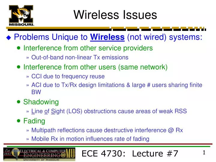
Wireless Issues. Problems Unique to Wireless (not wired) systems: Interference from other service providers Out-of-band non-linear Tx emissions Interference from other users (same network) CCI due to frequency reuse ACI due to Tx/Rx design limitations & large # users sharing finite BW

E N D
Wireless Issues • Problems Unique to Wireless (not wired) systems: • Interference from other service providers • Out-of-band non-linear Tx emissions • Interference from other users (same network) • CCI due to frequency reuse • ACI due to Tx/Rx design limitations & large # users sharing finite BW • Shadowing • Line of Sight (LOS) obstructions cause areas of weak RSS • Fading • Multipath reflections cause destructive interference @ Rx • Mobile Rx in motion influences rate of fading ECE 4730: Lecture #7
Wireless Issues • Wired Channel stationary & predictable • Wireless Channel random & unpredictable • Must be characterized in a statistical fashion • Field measurements often needed to characterize radio channel performance ** Mobile Radio Channel (MRC) has unique problems that limit performance of wireless systems *** ECE 4730: Lecture #7
Radio Signal Propagation • Two basic goals of propagation modeling: 1) Predict magnitude and rate (speed) of RSS fluctuations over short distances and/or time durations • “Short” typically a few land 10-100 milliseconds!! • RSS can vary by 30 to 40 dB!! • Small-scale RSS fluctuations fading (next chapter) 2) Predict average RSS for given Tx/Rx separation over km-scale distances • Characterize RSS over distances from 20 m to 20 km • Large-scale models • Needed to estimate coverage area of base station • Fig. 4.1, pg. 106 ECE 4730: Lecture #7
Radio Signal Propagation Small-scale RSS Large-scale RSS Indoor System ECE 4730: Lecture #7
Radio Signal Propagation • Wireless Link • Line of Sight (LOS) • Obstructed (OBS) • Basic Propagation Mechanisms • Free space • Reflection • Diffraction • Scattering ECE 4730: Lecture #7
Radio Signal Propagation • Free-Space Signal Propagation • Clear & unobstructed LOS path satellite and fixed microwave • Link transmission formula Rx power (Pr) vs. Tx-Rx separation (d) wherePt = Tx power (W) G = Tx or Rx antenna gain (unitless) relative to isotropic source far-field of antenna l= wavelength = c / f(m) L = system losses (antennas, T.L., atmosphere, etc.) unitless L = 1 for zero loss ECE 4730: Lecture #7
Large Scale Path Loss • Free-Space Path Loss (PL) in dB: • d2 power law relationship • Pr decreases at rate of 20 dB/decade of distance • e.g. Pr is 20 dB smaller @ 1 km vs. 100 m ECE 4730: Lecture #7
Large Scale Path Loss • Close in reference point (do) used in large-scale models wheredf : far-field distance of antenna = 2D2 / l D : largest linear dimension of antenna do : typically 100 m for outdoor systems and 1 m for indoor systems ECE 4730: Lecture #7
Large Scale Path Loss • Relating power to field strength: where o : free-space wave impedance = 120p = 377 W Ae : effective aperture of antenna = Gl2 / 4p ECE 4730: Lecture #7
Reflection • Reflections occur when RF energy incident upon boundary between two materials (e.g air/ground) with different electrical characteristics (m, e, s) • Reflecting surface must be large relative to l of RF energy • Reflecting surface must be smooth relative to l of RF energy • “Specular” reflection • Important reflecting surfaces for mobile radio: • Earth (ground) • Concrete streets • Buildings Walls/tinted windows/floors • Vehicles (metal surfaces) • Water (lakes, rivers, ponds, etc.) ECE 4730: Lecture #7
: incident field : reflected field : transmitted field qi: angle of incidence = 90° Snell’s Law qi = qr q i m2, e2, 2 m1, e1, 1 Reflection • Fresnel reflection coefficient G • Describes magnitude of reflected RF field strength • Depends upon material properties, polarization, & angle of incidence • Consider boundary between two materials: ECE 4730: Lecture #7
Reflection • Fresnel Reflection Coefficient • = wave impedance = • G is a measure of the discontinuity between electrical material properties • For free space : • e = eo = 8.85·10-12 F/m & m = mo = 4p·10-7 H/m • = o = = 377 W • For most materials mmo so that G depends largely on dielectric constant e • e = eo er + jewhere • er : relative dielectric constant • e: imaginary component ECE 4730: Lecture #7
Reflection • Imaginary component, e, of dielectric constant • e= 0 for “lossless” dielectric • e 0 for “lossy” dielectric transmitted energy undergoes attenuation due to absorption • Important for quantifying signal penetration thru walls/floors and into buildings • General G formulas 4.194.20 take into account polarization and angle of incidience (qi ) • **For small qi | G | approaches 1 total reflection** • For conductors (metals) | G | = 1 ECE 4730: Lecture #7
Ground Reflection Fig. 4.7, pg. 121 ECE 4730: Lecture #7
Ground Reflection Model • Ground Reflection (2-Ray) Model • results from combination of direct LOS path and ground reflected path** • Let be at reference point do then • Let direct path d=d’ and reflected path d = d” then • **assuming path to ground is LOS for both incident and reflected field ECE 4730: Lecture #7
Ground Reflection Model • Let direct path d = d’ and reflected path d = d” then • For large TxRx separation : qi 0 and G = 1 • Constructive/destructive interference can occur depending on phase difference between direct and reflected E fields • Phase differenceq due to path length difference, = d”d’, between and !! ECE 4730: Lecture #7
Ground Reflection Model • For d >> • and • d4 vs. d2 for free space !! • Pr1 / d4 or 40 dB/decade ECE 4730: Lecture #7
Ground Reflection • Two-ray path loss model: PL (dB)= 40 logd [10 logGt +10 logGr + 20 loght + 20 loghr] • For q = p = 180° d = 4ht hr/l • Vertical height difference between LOS & reflected path @ reflection point corresponds to first “Fresnel Zone” • Fresnel zone clearance used to determine if path is LOS or obstructed for point-to-point microwave systems ECE 4730: Lecture #7