Download
1 / 21
210 likes | 330 Views
Effects of partial measurement (non)invariance on manifest composite differences across groups. Holger Steinmetz Dep. of Work and Organizational Psychology University of Giessen / Germany Peter Schmidt Institute for Political Science University of Giessen / Germany. Introduction.

E N D
Effects of partial measurement (non)invariance on manifest composite differences across groups Holger Steinmetz Dep. of Work and Organizational Psychology University of Giessen / Germany Peter Schmidt Institute for Political Science University of Giessen / Germany
Introduction • Importance of analyses of mean differences For instance: • gender differences on wellbeing, self-esteem, abilities, behavior • differences between leaders and non-leaders on intelligence and personality traits • differences between cultural populations on psychological competencies, values, wellbeing • Usual procedure: t-test or ANOVA with observed composite scores • Latent variables vs. observed variables • Observed mean = indicator intercept + factor loading * latent mean • Research question: Effects of unequal intercepts and/or factor loadings across groups on composite differences
l1 d1 x1 l2 d2 x2 x l3 x3 d3 l4 x4 d4 Relationship between latent and observed means
xi l1 d1 x1 l2 d2 x2 x li l3 x3 d3 l4 ti x4 d4 x Relationship between latent and observed means
xi l1 d1 x1 l2 d2 x2 x li l3 x3 d3 l4 ti x4 d4 x Relationship between latent and observed means
x1 x2 x M(xi) x3 x4 k Relationship between latent and observed means xi l1 d1 l2 d2 li l3 d3 l4 ti d4 x
x1 x1 x2 x2 x x x3 x3 x4 x4 Group differences in intercepts and factor loadings Group A Group B xi M(xi) M(xi) M(xi) x k
x1 x1 x2 x2 x x x3 x3 x4 x4 Group differences in intercepts and factor loadings Group A Group B xi M(xi) M(xi) M(xi) x k
x1 x1 x2 x2 x x x3 x3 x4 x4 Group differences in intercepts and factor loadings Group A Group B xi M(xi) M(xi) M(xi) x k
Meaning of (unequal) intercepts • Associated terms used in the literature • Item bias • Differential item functioning • Measurement/factorial invariance („metric invariance", "scalar invariance") • Meaning • Response style (acquiescence, leniency, severity) • Response sets (e.g., social desirability) • Connotations of items • Item specific difficulty
The study • Partial invariance: Some loadings / intercepts are allowed to differ • Research question: Is partial invariance enough for composite mean difference testing? • Pseudo-differences • Compensation effects • Procedure (Mplus): • Step 1: a) Specification of two-group population models with varying differences in latent mean, intercepts and loadings b) 1000 replications, raw data saved • Step 2: Creation of a composite score • Step 3: Analysis of composite differences • Step 4: Aggregation (-> sampling distribution)
The study Group B Group A x1 x1 k=.00 k=.00 k=.30 • Population model: • Two groups • One latent variable • Conditions: • 4 vs. 6 indicators • Latent mean difference: 0 vs. .30 • Intercepts: equal vs. one vs. two intercepts unequal in varying directions (-.30 vs. +.30) • Loadings: equal (l‘s = .80) vs. one vs. two loadings = .60 • Sample size: 2x100 vs. 2x300 • Dependent variables • Average composite mean difference • Percent of significant composite differences x2 x2 x x x3 x3 x4 x4 x5 x5 l=.80 l=.60 x6 x6 t=.00 t=-.30
Pseudo-DifferencesEffects on the average composite difference 0.30 0.25 1 intercept unequal 2 intercepts unequal 0.20 0.15 0.10 0.05 0.00 4 Ind. 6 Ind. 4 Ind. 6 Ind. N = 2 x 100 N = 2 x 300
Pseudo-DifferencesEffects on the probability of significant differences (Type I error) 0.60 All intercepts equal 0.50 1 intercept unequal 2 intercepts unequal 0.40 0.30 0.20 0.10 0.00 4 Ind. 6 Ind. N = 2 x 100
Pseudo-DifferencesEffects on the probability of significant differences (Type I error) 0.60 All intercepts equal 0.50 1 intercept unequal 2 intercepts unequal 0.40 0.30 0.20 0.10 0.00 4 Ind. 6 Ind. 4 Ind. 6 Ind. N = 2 x 100 N = 2 x 300
Compensation effectsEffects on the average composite differences 0.30 All intercepts equal 1 intercept unequal 2 intercepts unequal 0.25 Effect of unequal loadings 0.20 Effect of unequal intercepts 0.15 0.10 0.05 0.00 2 Loadings unequal Loadings equal 1 Loading unequal 4 Indicators
Compensation effectsEffects on the average composite differences 0.30 All intercepts equal 1 intercept unequal 2 intercepts unequal 0.25 0.20 0.15 0.10 0.05 0.00 2 Loadings unequal 2 Loadings unequal Loadings equal 1 Loading unequal Loadings equal 1 Loading unequal 4 Indicators 6 Indicators
Compensation effectsEffects on the probability of significant differences (Power) 0.90 All intercepts equal 1 intercept unequal 0.80 2 intercepts unequal 0.70 0.60 0.50 0.40 0.30 0.20 0.10 0.00 2 Loadings unequal 2 Loadings unequal Loadings equal 1 Loading unequal Loadings equal 1 Loading unequal N = 2x100 / 4 Indicators N = 2x300 / 6 Indicators
Summary • Pseudo-differences • Even one unequal intercept increases the risk to find spurious composite differences • High sample size increases risk (up to 60% with two unequal intercepts) • Unequal factor loadings have only a low influence • Number of indicators reduces the risk – but not substantially • Compensation effects • Just one unequal intercept reduces the size of the composite difference to 50% • With a “small” sample size little chance to find a significant composite difference (power = .25 - .40) • Two unequal intercepts drastically reduce the composite difference: The power in the „best“ condition (2x300, 6 Ind.) is only .50
Conclusons • Most comparisons of means rely on traditional composite difference analysis • These methods make assumptions that are unrealistic (i.e., full invariance of intercepts and loadings) • Even minor violations of these assumptions increase the risk of drawing wrong conclusions • Advantages of SEM: • Assumptions can be tested • Partial invariance implies no danger • Greater power even in small samples
Thank you very much! Contact: Holger.Steinmetz@web.de