Download

1 / 38
380 likes | 513 Views
Stochastic Disagregation of Monthly Rainfall Data for Crop Simulation Studies. Stochastic disaggregation, and deterministic bias correction of GCM outputs for crop simulation studies. Amor VM Ines and James W Hansen International Institute for Climate Prediction

E N D
Stochastic Disagregation of Monthly Rainfall Data for Crop Simulation Studies Stochastic disaggregation, and deterministic bias correction of GCM outputs for crop simulation studies Amor VM Ines and James W Hansen International Institute for Climate Prediction The Earth Institute at Columbia University Palisades, NY, USA
Linkage to crop simulation models Crop simulation models (DSSAT) Daily Weather Sequence Seasonal Climate Forecasts Crop forecasts <<<GAP>>>
a) Stochastic disaggregation Crop simulation models (DSSAT) Monthly rainfall Stochastic disaggregation Weather Realizations GCM ensemble forecasts Stochastic weather generator Crop forecasts <<<Bridging the GAP>>>
b) Bias correction of daily GCM outputs Crop simulation models (DSSAT) 24 GCM ensemble members Bias correction of daily outputs Weather Realizations Crop forecasts <<<Bridging the GAP>>>
Objectives • To present stochastic disaggregation, and deterministic bias correction as methods for generating daily weather sequences for crop simulation models • To evaluate the performance of the two methods using the results of our experiments in Southeastern US (Tifton, GA; Gainesville, FL) and Katumani, Machakos Province, Kenya.
Part I. Stochastic disaggregation of monthly rainfall amounts
INPUT OUTPUT Structure of a stochastic weather generator (Begin next day) f(u) Generate uniform random number Generate today’s non-ppt. variables u Generate ppt.=0 Dry-day non-ppt. parameters: μk,0; σk,0 u<=pc? pc=p01 f(x) Generate a non-zero ppt. Wet-day non-ppt. parameters: μk,1; σk,1 pc=p11 x Precipitation sub-model Non-precipitation sub-model (after Wilks and Wilby, 1999)
Precipitation sub-model Occurrence model: p01=Pr{ppt. on day t | no ppt. on day t-1} Markovian process p11=Pr{ppt. on day t | ppt. on day t-1} Intensity model: Mixed-exponential f(x)=α/β1 exp[-x/β1] + (1-α)/β2 exp[-x/β2] μ= αβ1 + (1-α)β2 Max. Likelihood (MLH) σ2= αβ12 + (1-α)β22 + α(1-α)(β1-β2)
Long term rainfall frequency: π=p01/(1+p01-p11) First lag auto-correlation of occurrence series: r1=p11-p01
Temperature and radiation model Trivariate 1st order autoregressive conditional normal model z(t)=[A]z(t-1)+[B]ε(t) zk(t)=ak,1z1(t-1)+ak,2z2(t-1)+ak,3z3(t-1)+ bk,1ε1(t)+bk,2ε2(t)+bk,3ε3(t) μk,0(t)+σk,0zk(t); if day t is dry Tk(t)= μk,1(t)+σk,1zk(t); if day t is wet NOTE: Used long-term conditional means of TMAX,TMIN,SRAD
Decomposing monthly rainfall totals Rm =μ x π Dimensional analysis: where: Rm - mean monthly rainfall amounts, mm d-1 μ - mean rainfall intensity, mm wd-1 π - rainfall frequency, wd d-1
Conditioning weather generator inputs we condition α in the intensity model μ = Rm /π we condition p01, p11 from the frequency and auto-correlation equations π = Rm / μ …and other higher order statistics
Conditioning weather generator outputs First step: Iterative procedure - by fixing the input parameters of the weather generator using climatological values, generate the best realization using the test criterion |1-RmSim/Rm|j <= 5% Second step: Rescale the generated daily rainfall amounts at month j by (Rm/RmSim)j
Applications A.1 Diagnostic case study • Locations: Tifton, GA and Gainesville, FL • Data: 1923-1999 A.2 Prediction case study • Location: Katumani, Kenya • Data: MOS corrected GCM outputs (ECHAM4.5) • ONDJF (1961-2003)
Simulation Data(Tifton, GA and Gainesville, FL) Crop Model: CERES-Maize in DSSATv3.5 Crop: Maize (McCurdy 84aa) Sowing dates: Apr 2 1923 – Tifton Mar 6 1923 – Gainesville Soils: Tifton loamy sand #25 – Tifton Millhopper Fine Sand – Gainesville Soil depth: 170cm; Extr. H2O:189.4mm – Tifton 180cm; Extr. H2O:160.9mm – Gainesville Scenario: Rainfed Condition Simulation period: 1923-1996
A.1 Diagnostic Case Sensitivity of RMSE and correlation of yield π μ Rm Tifton, GA Gainesville, FL
Gainesville, FL Sensitivity of RMSE and R of rainfall amount, frequency and intensity at month of anthesis (May) π μ Rm μ π Rm
μ 1000 Realizations π Gainesville, FL Rm Predicted Yields
A.2 Case study: Katumani, Machakos Province, Kenya Skill of the MOS corrected GCM data OND
Simulation Data(Katumani, Machakos Province, Kenya) Crop Model: CERES-Maize Crop: Maize (KATUMANI B) Sowing dates (Nov 1 1961) Soil depth :130cm Extr. H2O:177.0mm Scenario: Rainfed Simulation period: 1961-2003 Sowing strategy: conditional-forced
Sensitivity of RMSE and correlation of yield Rm (Hindcast) Rm+π2 π2 (Hindcast) π1 (Conditioned)
Rm (Hindcast) π2 (Hindcast) π1 (Conditioned) Rm+ π2
Part II. Bias correction of daily GCM outputs (precipitation)
Statement of the problem Rm Climatology, Monthly rainfall
Rm Variance, Monthly rainfall
μ Intensity π Frequency
Proposed bias correction (a)-correcting frequency (b)-correcting intensity
Application Location: Katumani, Machakos, Kenya Climate model: ECHAM4.5 (Lat. 15S;Long. 35E) Crop Model: CERES-Maize Crop: Maize (KATUMANI B) Sowing dates (Nov 1 1970) Soil depth :130cm; Extr. H2O:177.0mm Scenario: Rainfed Simulation period: 1970-1995 Sowing strategy: conditional-forced
Results Rm μ Variance, Rm Variance, μ
Comparison of yield predictions using disaggregated, MOS-corrected monthly GCM predictions, and bias-corrected daily gridcell GCM simulations
μ Bias corrected seasonal rainfall (OND) π Rm
Comparison of MOS corrected and bias corrected seasonal rainfall (OND)
Why are we successful? Is the procedure applicable in every situation? Inter-annual correlation (R) of monthly rainfall
Conclusions • Stochastic disaggregation: • Conditioning the outputs to match target monthly rainfall totals works better than conditioning the inputs of the weather generator: • i) it tends to minimize the variability of monthly rainfall within realizations; • ii) tends to reproduce better the historic intensity and frequency; • iii) requires fewer realizations to achieve a given level of accuracy in crop yield prediction
Deterministic bias correction of daily GCM precip: • There are useful information hidden in daily GCM outputs • Extracting them entails interpreting the data according to the GCM climatology then correcting them based on observed climatology • Overall, the success of stochastic disaggregation or bias correction of GCM outputs for crop yield prediction depends greatly on the skill of the GCM THANK YOU…