Download
1 / 17
170 likes | 271 Views
I. I. r. B =. 2 r. . . . . B. H =. . I. =. 2 r. 16.360 Lecture 3. Last lecture:. Magnetic field by constant current. = r 0 ,. r: relative magnetic permeability. r =1 for most materials. 16.360 Lecture 3. Last lecture:. Traveling wave.

E N D
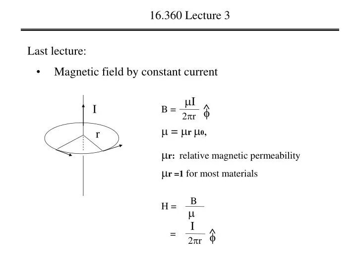
I I r B = 2r B H = I = 2r 16.360 Lecture 3 Last lecture: • Magnetic field by constant current = r 0, r: relative magnetic permeability r =1 for most materials
16.360 Lecture 3 Last lecture: • Traveling wave y(x,t) = Acos(2t/T-2x/), y(x,t) = Acos(x,t), (x,t) = 2t/T-2x/,
16.360 Lecture 3 Last lecture: • Traveling wave y(x,t) = Acos(2t/T+2x/), Velocity = 0.6/0.6T = /T Phase velocity: Vp = dx/dt = - /T
Vs(t) VC(t) i (t) i(t)dt/C, VC(t) = 16.360 Lecture 3 • Phasor VR(t) Vs(t) = V0Sin(t+0), VR(t) = i(t)R, Vs(t) = VR(t) +VC(t), V0Sin(t+0) = i(t)dt/C + i(t)R, Integral equation, Using phasor to solve integral and differential equations
jt ) Z(t) = Re( Z e Z is time independent function of Z(t), i.e. phasor jt jt e e = Re(V ), j(0 - /2) , V = V0 e 16.360 Lecture 3 • Phasor Vs(t) = V0Sin(t+0) j(0 - /2) ) = Re(V0 e
jt ) i(t) = Re( I e 1 jt )/C + = Re(I i(t)dt= Re( I e )dt j jt jt jt e e e jt ), Re( I e Re(V ) 16.360 Lecture 3 • Phasor 1 ), = Re(I j time domain equation: V0Sin(t+0) = i(t)dt/C + i(t)R, phasor domain equation:
jt 1 = I ) i(t) = Re( I e jC V j(0 - /2) j(0 - /2) V0 e V0 e 16.360 Lecture 3 • Phasor domain V + I R , I = R + 1/(jC) = , R + 1/(jC) Back to time domain: jt e = Re ( ) R + 1/(jC)
16.360 Lecture 3 • An Example : VR(t) Vs(t) = V0Sin(t+0), VR(t) = i(t)R, Vs(t) VL(t) i (t) Ldi(t)/dt, VL(t) = Vs(t) = VR(t) +VL(t), V0Sin(t+0) = Ldi(t)/dt + i(t)R, differential equation, Using phasor to solve the differential equation.
jt ) i(t) = Re( I e jt jt jt e e e jt ), Re( I e Re(V ) 16.360 Lecture 3 • Phasor jt di(t)/dt= Re(d I e )/dt j = Re(I ), time domain equation: V0Sin(t+0) = Ldi(t)/dt + i(t)R, phasor domain equation: j )L + = Re(I
jt ) i(t) = Re( I e V j(0 - /2) j(0 - /2) V0 e V0 e 16.360 Lecture 3 • Phasor domain jL + I R V = I , I = R + (jL) = , R + jL) Back to time domain: jt e = Re ( ) R + (jL)
16.360 Lecture 3 • Steps of transferring integral or differential equations to linear • equations using phasor. • Express time-dependent variables as phsaor. • Rewrite integral or differential equations in phasor domain. • Solve phasor domain equations • Change phasors variable to their time domain value
16.360 Lecture 3 • Electromagnetic spectrum. Recall relation: f = v. • Some important wavelength ranges: • Fiber optical communication: = 1.3 – 1.5m. • Free space communication: ~ 700nm – 980nm. • TV broadcasting and cellular phone: 300MHz – 3GHz. • Radar and remote sensing: 30GHz – 300GHz
16.360 Lecture 3 • Transmission lines • Transmission line parameters, equations • Wave propagations • Lossless line, standing wave and reflection coefficient • Input impedence • Special cases of lossless line • Power flow • Smith chart • Impedence matching • Transients on transmission lines
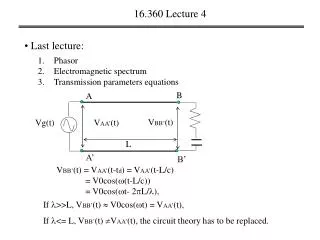
16.360 Lecture 3 • Today • Transmission line parameters, equations B A VBB’(t) Vg(t) VAA’(t) L A’ B’ VAA’(t) = Vg(t) = V0cos(t), Low frequency circuits: VBB’(t) = VAA’(t) Approximate result VBB’(t) = VAA’(t-td) = VAA’(t-L/c) = V0cos((t-L/c)),
B A VBB’(t) Vg(t) VAA’(t) L A’ B’ 16.360 Lecture 3 • Transmission line parameters, equations Recall: =c, and = 2 VBB’(t) = VAA’(t-td) = VAA’(t-L/c) = V0cos((t-L/c)) = V0cos(t- 2L/), If >>L, VBB’(t) V0cos(t) = VAA’(t), If <= L, VBB’(t) VAA’(t), the circuit theory has to be replaced.
16.360 Lecture 3 • Next lecture • Types of transmission lines • Lumped-element model • Transmission line equations • Wave propagation