Download
1 / 62
2.04k likes | 4.64k Views
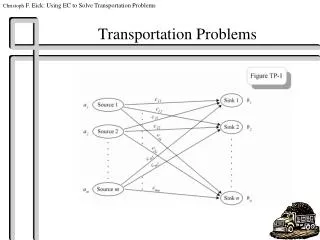
TRANSPORTATION PROBLEMS . Introduction . Transportation problem is a special kind of LP problem in which objective is to transport various quantities of a single homogenous commodity, to different destinations in such a way that the total transportation cost is minimized. Examples:. Sources

E N D
Introduction Transportation problem is a special kind of LP problem in which objective is to transport various quantities of a single homogenous commodity, to different destinations in such a way that the total transportation cost is minimized.
Examples: • Sources factories, finished goods warehouses , raw materials ware houses, suppliers etc. • Destinations Markets Finished goods ware house raw materials ware houses, factories,
Terminology Used • Feasible Solution – Non negative values of xij, where i=1,2,..,m and j=1,2,..,n which satisfy the constraints of supply & demand is called feasible to the solution. • Basic Feasible Solution – A feasible solution to a m origin and n destination problem is said to be basic if no. of positive allocations = m+n-1. • Optimal Feasible Solution – A feasible solution is said to be optimal if it minimizes the total transportation cost. The optimal solution itself may or may not be a basic solution. After this no further decrease in transportation cost is possible.
Balanced Transportation Problem – A transportation problem in which the total supply from all sources equals the total demand in all destinations • Unbalanced Transportation Problem – such problems which are not balanced • Matrix Terminology
Assumptions of the model • Availability of the quantity. • Transportation of items. • Cost per unit. • Independent cost. • Objective.
1 2 j n Supply a1 a2 ai am 1 2 i m S O U R C E i • Destination j Demand b1 b2bjbn
Where, • m- number of sources • n- number of destinations • ai- supply at source I • bj – demand at destination j cij – cost of transportation per unit from source i to destination j Xij – number of units to be transported from the source i to destination j
Steps to solve a Transportation Model • Formulate the problem and setup in the matrix form. • Obtain the Initial basic Feasible Solution. • Test the initial solution for optimality. • Updating the solution.
Factories (Sources) Warehouses (Destinations) 100 Units D A 300 Units 300 Units E B 200 Units 300 Units F C 200 Units Transportation problem with 3 sources and 3 destinations Capacities Shipping Routes Requirements
Setting Up a Transportation Problem • The first step is setting up the transportation table • Its purpose is to summarize all the relevant data and keep track of algorithm computations Transportation costs per desk for Executive Furniture
Setting Up a Transportation Problem D’s capacity constraint • Transportation table for Executive Furniture Cell representing a source-to-destination (E to C) shipping assignment that could be made Total supply and demand Cost of shipping 1 unit from F factory to B warehouse C warehouse demand
North West Corner Method (NWCM) • Construct an empty m х n matrix, completed with rows and columns. • Indicate the row totals and column totals at the end. • Starting with (1,1) cell at the North-West Corner of the matrix, allocate maximum possible quantity keeping in view that allocation can neither be more than the quantity required by the respective warehouses nor more than the quantity available at each supply centre.
Adjust the supply and demand numbers in the respective rows and column allocations. • If the supply for the first row is exhausted then move down to the first cell in the second row and first column and go to step 4. • If the demand for first column is satisfied, then move to the next cell in the second column and first row and go to step 4. • If for any cell, supply equals demand then the next allocation can be made in cell either in the next row or column. • Continue the procedure until the total available quantity is fully allocated to the cells as required.
Developing an Initial Solution: Northwest Corner Rule • Beginning in the upper left hand corner, we assign 100 units from D to A. This exhaust the supply from D but leaves A 200 desks short. We move to the second row in the same column.
Developing an Initial Solution: Northwest Corner Rule • Assign 200 units from E to A. This meets A’s demand. E has 100 units remaining so we move to the right to the next column of the second row.
Developing an Initial Solution: Northwest Corner Rule • Assign 100 units from E to B. The E supply has now been exhausted but B is still 100 units short. We move down vertically to the next row in the B column.
Developing an Initial Solution: Northwest Corner Rule • Assign 100 units from F to B. This fulfills B’s demand and F still has 200 units available.
Developing an Initial Solution: Northwest Corner Rule • Assign 200 units from Fort Lauderdale to Cleveland. This exhausts Fort Lauderdale’s supply and Cleveland’s demand. The initial shipment schedule is now complete.
Developing an Initial Solution: Northwest Corner Rule • We can easily compute the cost of this shipping assignment • This solution is feasible but we need to check to see if it is optimal
Lowest Cost Entry Method OR Matrix Minima Method • Select the cell with the lowest transportation cost among all the rows or columns of the transportation table. If the minimum cost is nor unique the select arbitrarily any cell with the lowest cost. • Allocate as many units as possible to the cell determined in step 1 and eliminate that row in which either capacity or requirement is exhausted. • Adjust the capacity and requirement for the next allocations. • Repeat steps 1 to 3 for the reduced table until the entire capacities are exhausted to fill the requirement at different destinations.
An example for Lowest Cost Entry MethodStep 1: Select the cell with minimum cost.
Step 3: Find the new cell with minimum shipping cost and cross-out row 2
Step 4: Find the new cell with minimum shipping cost and cross-out row 1
Step 5: Find the new cell with minimum shipping cost and cross-out column 1
Step 6: Find the new cell with minimum shipping cost and cross-out column 3
Step 7: Finally assign 6 to last cell. The bfs is found as: X11=5, X21=2, X22=8, X31=5, X33=4 and X34=6
Vogel’s Approximation Method (VAM) Considered as the best method. The steps are as follows: • For each row of the table identify the lowest and the next lowest cost cell. Find their differences and place it to the right of that row. In case two cells contain the same least cost then the difference shall be zero. • Similarly find the difference of each column and place it below each column. These differences found in step 2 & 3 are also called penalties.
Looking at all the penalties, identify highest of them and the row or column relative to that penalty. Allocate the maximum possible units to the least cost cell in the selected row or column. Ties should be broken in this order Maximum difference least cost cell Maximum difference tie Least Cost Cell. Maximum Units allocation tie Arbitrary. • Adjust the supply & demand and cross the satisfied row or column. • Recompute the column and row differences ignoring deleted row/columns and go to step 3. repeat the procedure until all the column and row totals are satisfied.
Step 2: Identify the largest penalty and assign the highest possible value to the variable.
Step 3: Identify the largest penalty and assign the highest possible value to the variable.
Step 4: Identify the largest penalty and assign the highest possible value to the variable.
Step 5: Finally the bfs is found as X11=0, X12=5, X13=5, and X21=15
Optimality Test by MODI Method • Construct the transportation table with given cost of transportation and rim conditions. • Determine initial basic feasible solution using a suitable method. • For occupied cells, calculate Ri and Kj for rows and columns respectively, where Cij = Ri + Kj • For occupied cells, the opportunity cost is calculated using formula dij = Cij – (Ri + Kj) • Now, the opportunity cost of unoccupied cells is determined, where Opportunity cost = Actual cost – Implied Cost dij = Cij – (Ri + Kj)
Examine unoccupied cells evaluation for dij • if dij > 0, cost will increase, i.e. optimal solution has arrived. • If dij = 0, cost will remain unchanged but there exists an alternate solution. • If dij < 0, then improved solution can be obtained by moving to step 7. • Select an unoccupied cell with largest negative opportunity cost among all unoccupied cells. • Construct a closed path for unoccupied cell determined in step7 and assign (+) and (-) sign alternatively beginning with plus sign for the selected unoccupied cell in any direction. • Assign as many units as possible to the unoccupied cell satisfying rim conditions. The smallest allocation in a cell with negative sign on the closed path indicated the number of units that can be transported to the unoccupied cells. This quantity is added to all the occupied cells on the path marked with plus sign and substracted from those occupied cells on the path marked with minus sign. • Go to step 4 and repeat procedure until all dij > 0,i.e., an optimal solution is reached.
Stepping-Stone Method: Finding a Least Cost Solution • The stepping-stone method is an iterative technique for moving from an initial feasible solution to an optimal feasible solution • There are two distinct parts to the process • Testing the current solution to determine if improvement is possible • Making changes to the current solution to obtain an improved solution • This process continues until the optimal solution is reached
Occupied shipping routes (squares) Number of rows Number of columns = + – 1 Stepping-Stone Method: Finding a Least Cost Solution • There is one very important rule • The number of occupied routes (or squares) must always be equal to one less than the sum of the number of rows plus the number of columns • In the Executive Furniture problem this means the initial solution must have 3 + 3 – 1 = 5 squares used • When the number of occupied rows is less than this, the solution is called degenerate
Testing the Solution for Possible Improvement • The stepping-stone method works by testing each unused square in the transportation table to see what would happen to total shipping costs if one unit of the product were tentatively shipped on an unused route • There are five steps in the process
Five Steps to Test Unused Squares with the Stepping-Stone Method • Select an unused square to evaluate • Beginning at this square, trace a closed path back to the original square via squares that are currently being used with only horizontal or vertical moves allowed • Beginning with a plus (+) sign at the unused square, place alternate minus (–) signs and plus signs on each corner square of the closed path just traced
Five Steps to Test Unused Squares with the Stepping-Stone Method • Calculate an improvement index by adding together the unit cost figures found in each square containing a plus sign and then subtracting the unit costs in each square containing a minus sign • Repeat steps 1 to 4 until an improvement index has been calculated for all unused squares. If all indices computed are greater than or equal to zero, an optimal solution has been reached. If not, it is possible to improve the current solution and decrease total shipping costs.
Five Steps to Test Unused Squares with the Stepping-Stone Method • For the Executive Furniture Corporation data Steps 1 and 2. Beginning with Des Moines–Boston route we trace a closed path using only currently occupied squares, alternately placing plus and minus signs in the corners of the path • In a closed path, only squares currently used for shipping can be used in turning corners • Only one closed route is possible for each square we wish to test
Five Steps to Test Unused Squares with the Stepping-Stone Method Step 3. We want to test the cost-effectiveness of the Des Moines–Boston shipping route so we pretend we are shipping one desk from Des Moines to Boston and put a plus in that box • But if we ship one more unit out of Des Moines we will be sending out 101 units • Since the Des Moines factory capacity is only 100, we must ship fewer desks from Des Moines to Albuquerque so we place a minus sign in that box • But that leaves Albuquerque one unit short so we must increase the shipment from Evansville to Albuquerque by one unit and so on until we complete the entire closed path
Warehouse A Warehouse B $5 $4 FactoryD 100 $4 $8 FactoryE 100 200 Five Steps to Test Unused Squares with the Stepping-Stone Method • Evaluating the unused Des Moines–Boston shipping route – + – +
99 1 99 201 Five Steps to Test Unused Squares with the Stepping-Stone Method Warehouse A Warehouse B $5 $4 • Evaluating the unused Des Moines–Boston shipping route FactoryD 100 – + – + $4 $8 FactoryE 100 200
Warehouse A Warehouse B $5 $4 99 FactoryD 1 100 – + – + $4 $8 99 201 FactoryE 100 200 Result of Proposed Shift in Allocation = 1 x $4 – 1 x $5 + 1 x $8 – 1 x $4 = +$3 Five Steps to Test Unused Squares with the Stepping-Stone Method • Evaluating the unused Des Moines–Boston shipping route
Des Moines–Boston index = IDB = +$4 – $5 + $5 – $4 = + $3 Five Steps to Test Unused Squares with the Stepping-Stone Method Step 4. We can now compute an improvement index (Iij) for the Des Moines–Boston route • We add the costs in the squares with plus signs and subtract the costs in the squares with minus signs • This means for every desk shipped via the Des Moines–Boston route, total transportation cost will increase by $3 over their current level
Five Steps to Test Unused Squares with the Stepping-Stone Method Step 5. We can now examine the Des Moines–Cleveland unused route which is slightly more difficult to draw • Again we can only turn corners at squares that represent existing routes • We must pass through the Evansville–Cleveland square but we can not turn there or put a + or – sign • The closed path we will use is + DC – DA + EA – EB + FB – FC